Second Humanoid, Nanotechnology, Information, Communication and Control, Environment and Management (HNICEM) International Conference The Institute of Electrical and Electronics Engineers Inc. (IEEE) – Philippine Section March 17-20, 2005, HYATT Regency Hotel, Manila, Philippines
Heuristic Parameter Estimation Methods for S-System Models of Biochemical Networks Prospero C. Naval, Jr.
Orland R. Gonzalez
Department of Computer Science
Department of Computer Science
University of the Philippines-Diliman
[email protected]
University of the Philippines-Diliman
Eduardo Mendoza Department of Mathematics University of the Philippines-Diliman
[email protected]
Luis G. Sison Department of Electrical & Electronics Engineering University of the Philippines-Diliman
[email protected]
Physics Dept & Center for NanoScience Ludwig Maximillians University-Munich
[email protected] ABSTRACT Advanced NMR and mass spectroscopy permit simultaneous measurements of time-course in-vivo metabolite concentrations within an organism. These metabolic profiles are loaded with structural and kinetic information regarding the biochemical networks from which they were drawn. Extracting these information will require systematic application of both experimental and computational techniques. S-systems are non-linear dynamical models based on the power-law formalism which provide a general framework for the simulation of integrated biochemical systems exhibiting complex dynamics such those present in genetic circuits, immune and metabolic networks. In this paper we describe complementary heuristic methods for recovering the parameters of S-systems from time-course biochemical data. Keywords Bioinformatics, S-System Parameter Estimation, Simulated Annealing, Evolutionary Multiobjective Optimization 1. INTRODUCTION The living cell is a complex system whose survival, growth, and reproduction all depend on thousands of biochemical reactions. Metabolism extracts energy from nutrients and provides building blocks for cellular structures necessary for repair and reproduction. Metabolic
reactions are highly orchestrated biochemical reactions that are modulated by enzymes that accelerate and modulate reaction rates. Understanding the dynamics of a biochemical system often consists in postulating a model for simulation which allows the experimentalist to answer “what if” questions, explore possible system faults, and predict actual system behavior. Biochemical reasoning, including the ability to predict and manipulate biochemical behavior to increase yield or reduce unwanted by-products is central to bioprocess engineering. Modeling of metabolic pathways are starting to yield new insights on the nature of certain diseases and their possible treatments [3]. Biochemical Systems Theory (BST) is a general framework for modeling and analyzing biochemical systems. Biochemical properties and dynamics suggest a convenient nonlinear dynamical system assuming the power law forms
+ ! X& i = Vi ! Vi i = 1, 2,..., n gi ,n+1 gi , n + m g g g + Vi = # i X 1 i1 X 2 i 2 L X n in X n+1 L X n+ m hi ,n+1 hi ,n+ m h h h ! Vi = " i X 1 i1 X 2i 2 L X nin X n+1 L X n+ m where the terms
Vi + and Vi! represent production and
depletion processes respectively. Variables X i (t ) describe the state of dependent variables for constituents
i = 1, 2, K , n and for all time points of interest. Dependent variables stand for metabolites whose concentrations vary significantly during an experiment. Independent variables, on the other hand, are those that vary little that they may be considered constant. Enzymes are usually treated as independent variables. In our notation, all variables X i (t ) whose indices ranges from i = 1, 2, K , n are the dependent variables while the independent variables whose indices assume values i = n + 1, K , n + m . Numerous authors (e.g. [13] [10], etc.) have argued for the S-System formulation
n+ m gij n+ m hij X& i = $ i ! X j " # i ! X j j =1 j =1 where ! i and ! i represent the rates at which the concentrations of X i increase and decrease respectively,
g ij and hij are the kinetic orders of the reactions. Positive kinetic order values mean activating influences and negative values indicate inhibition. 2. THE PARAMETER ESTIMATION PROBLEM The inverse problem of recovering the rate constants and kinetic order parameters of an S-System model is vital to the development of simulation models which will eventually lead to a deeper understanding of metabolic processes. There are two approaches for determining the parameters of an S-System model The first estimates parameters based on how a biochemical system responds to small perturbations around the steady state. Estimation from dynamic data, on the other hand, requires measurements of all dependent variables at sequential points in time. The data reflects transient response of the system after some perturbations from the steady state. The goal of S-System parameter estimation is to recover the set of parameters that produced time-course data X i , i = 1,2, K , n . In metabolic profiling, we are provided with metabolic concentrations of the metabolites at many sequential time points and the challenge is to infer the parameters " i , ! i , g ij , hij of the underlying pathway. S-System parameter estimation has been investigated by a number of researchers in the past. Voit and Savageau used non-linear regression to optimize the production of ethanol in yeast culture [15]. Sorribas and Cascante examined to what extent the metabolic pathway could be inferred from steady state data [11]. Genetic Algorithms were used by Zhang et. al. [16] to estimate the parameters for S-Systems describing palm oil. Okamoto et. al [8], Akutsu et. al. [1], Maki et. al. [6], and Sakamoto et. al. [9] likewise used Genetic Algorithms for estimating the SSystem parameters in gene-regulatory systems.
However, success remains limited only to systems whose underlying variables are small in number and when data points are abundant. Another challenge commonly encountered is that multiple sets of solutions often have the same residual error with respect to the data set and there is little guidance on the qualitative difference among them. The most significant challenge remains that of nonconvergence due to the abundance of local minima. In this paper, we propose two complementary heuristic parameter estimation methods: Simulated Annealing and Evolutionary Multiobjective Optimization (EMOO). For S-Systems, heuristic methods can locate the vicinity of the global solutions efficiently but global optimality is not guaranteed. Simulated Annealing optimizes a single objective to arrive at a single solution with great efficiency. Evolutionary Multiobjective Optimization makes use of several objectives and makes decisions based on the preferences given. At each step, the optimizer selects candidate solutions on the basis of alternative trade-offs specified by objective function values. Once the S-System parameters have been recovered from experimental data, the mathematical model is subjected to some tests to confirm its consistency and realism [13]. Steady state analysis is performed to check if the model has the observed steady state. The system's robustness to perturbation is verified through local stability, metabolite and flux gain sensitivity analyses. In our proposed Evolutionary Multiobjective Optimization approach, all these tests are incorporated as objectives and constraints that the optimizer must consider in choosing the candidate solution. The experimentalist's task of performing the analyses himself/herself is thus reduced. 3. REGRESSION BY SIMULATED ANNEALING We propose a Simulated Annealing-based Parameter Estimation procedure that follows the iterative estimateprune-estimate strategy (outlined in Figure 1 used by other authors [14]. The first step involves the formulation of the complete symbolic S-system model. Knowing the number of dependent and independent constituents in the system being modeled is sufficient to perform this step. Next, a priori information regarding the structure of the system in question may be used to reduce the complete S-system symbolic formulation in order to help the upcoming regression step. This type of information may or may not be available at the start. After the symbolic formulation has been constructed, a candidate solution is obtained from a given biochemical profile using simulated annealing.
out completely but are accepted with a probability proportional to this pseudo-temperature.
Figure 1: Estimation Flow Diagram
The candidate solution in the form of a set of specific values for each of the system parameters is then evaluated for its acceptability. If found acceptable, the candidate is added to the set of candidate solutions. Otherwise, it is rejected in preparation for another regression step. Finally, after the pool of acceptable candidate solutions has been created, the best solution is selected based on certain criteria such as which solution makes the most biological sense. A priori information regarding the properties of the system being modeled may be used to constrain the initial search space. We utilize for our initial constraints only those which are based on properties commonly observed in most realistic biochemical systems. The first such constraint based on general knowledge on the field [13] is the restriction of kinetic orders to the closed range [-2.0, 2.0]. The next two constraints which were also used by other authors [14] is the setting of the g ii 's to zero and restriction of the hii 's to positive values. The regression step in the parameter estimation strategy is done with an optimization technique called Simulated Annealing (SA) which operates in way roughly analogous to how metal and glass are made. Simulated annealing differs from most other iterative improvement techniques in that it accepts candidate solutions that are of lower quality than the one it already has depending on the pseudo-temperature. In SA, inferior solutions are not ruled
Figure 2: Pseudocode for Simulated Annealing
The basic algorithm of Simulated Annealing we applied to S-systems parameter estimation is outlined in Figure 2. The technique starts with the creation of an initial estimate h which is simply an assignment of random values to all the parameters satisfying the initial constraints. This step corresponds to line 1 in the pseudocode. Line 3 involves the initialization of the control variable T which in analogy with real world annealing pertains to temperature. This initial value should be enough to "melt" the estimate. The rest of the lines 4-18 form a loop structure wherein the initial guess is iteratively refined in an effort to obtain better solutions. What follows are two desirable properties of simulated annealing which make it ideal for regression in a highly nonlinear error space such as that of S-systems parameter estimation [5]: •
Differs from most other iterative improvement techniques in that in SA transitions out of a local optimum are always possible at nonzero temperature.
•
An adaptive divide-and-conquer mechanism implicitly occurs. Gross features of the eventual
state of the system appear at higher temperatures while the finer details develop at lower temperatures. Essential to simulated annealing is the manner of randomly perturbing a given candidate solution. Perturbation was done by adding to each of the hypothesis' parameters a random value taken from a Gaussian distribution, that is,
p = p + c " N( µ , ! )
(1)
where p is the parameter, c is a constant, N( µ , ! ) is a function that returns a random number from a Gaussian distribution with mean µ and standard deviation ! . For our experiments, µ was fixed at 0.0 and ! at 1.0.
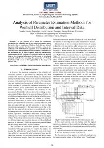
Figure 3: A generic branched network with four dependent constituents X 1 through X 4 , one constant source X 5 , and two regulatory signals (adapted from Voit and Almeida 2004 [14]).
4. SIMULATED ANNEALING RESULTS The strategy suggested in the previous section was tested using the same theoretical system Voit and Almeida used to illustrate their decoupling technique [14]. The system illustrated in Figure 3 is a generic branched network with four dependent constituents X 1 through X 4 , one constant source X 5 , and two regulatory signals. A typical numerical S-
system representation of this system is
X& 1 = 20 X 3!0.8 X 5 ! 10 X 10.5 X& 2 = 8 X 0.5 ! 3 X 0.75 1
2
X& 3 = 3 X 20.75 ! 5 X 30.5 X 40.2 X& 4 = 2 X 20.5 ! 6 X 40.8 X& = 0.9
X 1 (t 0 ) = 5.6 X 2 (t 0 ) = 3.1 X 3 (t 0 ) = 2.9
(2)
X 4 (t 0 ) = 3.1
5
We used this S-system model to create an artificial dataset with four sets of traces. These sets where formatted such that each one would resemble a biochemical profile. The graphical representation of one of these four is depicted in Figure 4. Using the parameter estimation strategy outlined in Figure 1, the artificial dataset was used to estimate the parameters of the theoretical system. The graph of this set superimposed with that of the true solution using one of the 4 initial conditions used to create the dataset is shown in Figure 5. Though the graphs of the initial estimated set were very close to those of the true solution for the initial conditions used in the dataset, observe that the parameters themselves are significantly different. Moreover, the similarities with the trace graphs do not necessarily hold for all initial conditions other than those used to create the dataset. This is the reason why subsequent rounds of pruning are important after initial results are retrieved. The actual parameter values of the final estimated set are very close with those of the true solution.
Figure 4: One of the four sets of traces in the dataset. Each was formatted to resemble biochemical profiles.
So far, estimation has only been done through traditional curve fitting using solutions to ODEs. The problem with this type of approach is that numerical integration needs a lot of computational power. Considering that contemporary regression techniques require error function evaluations of the error tens or even hundreds of thousands of times, the amount of time needed even with a powerful computer will be very substantial. Moreover, encountering stiff computations along the search may complicate the matter even further. In order for regression algorithms to cope with the scope and size of realistic biochemical systems, additional measures will have to be taken. Ameliorating the problem of heavy computational requirements due to numerical integration can be done in various ways. One way is to estimate each equation in the system with another differential equation that is easier to solve. However, this approach is quite limited in our inverse problem of parameter estimation since the system of ODEs changes dynamically. This is why as an alternative, some researchers have suggested the use of
techniques that approximate the temporal values of the differential equations directly from the data [14]. Not only will the system of ODEs be decoupled, numerical integration can be done away with altogether. In this research, we used for our decoupling procedure the approximation of the temporal values of the ODEs using the 3-point technique popular in engineering. The previous dataset which consisted of traces of timepoints was converted to sets of algebraic equations, one for each constituent. Because the system is now decoupled, the parameters of (1) no longer needed to be estimated as a system. Rather, it can now be done per differential equation X& i . Using the decoupling procedure described above, the parameters of (2) were once again estimated. Estimating the parameters of X& 1 took 2 pruning steps, X& 2 took 1 pruning step, X& took 2 pruning steps, and X& took 1 3
4
pruning step. Initial experiments described in this section were performed using 1.2GHz Athlon-XP machines had running times ranging anywhere from 20 to 30+ hours. The scale of the systems that can be handled can be increased through the employment of techniques that decouple systems of ODEs [14]. These additional procedures produced dramatic reductions in running times from the 20+ hours range to under 15 minutes. 5. AN EVOLUTIONARY MULTIOBJECTIVE APPROACH We propose an evolutionary multiobjective approach to the S-System parameter estimation problem. Evolutionary Multiobjective Optimization (EMOO) allows the experimentalist to combine and optimize on several objectives. The estimation problem may be seen as a search for solutions guided not only by minimization of residual error on data but also on other factors such as •
local stability of the biochemical system
•
how close are the estimated steady state concentrations to the actual experimental values
•
how much time the molecule remains in the pathway (transition time)
•
how sensitive are the metabolites with respect to changes in rate constants and kinetic orders.
EMOO provides sets of solutions that are optimal in the multiobjective sense. These Pareto-optimal solutions are optimal in all the objectives in that any further improvement in one implies degradation with respect to another.
One motivation for taking a multiobjective approach is the observation that in living organisms the underlying biochemical system is robust to changes in metabolite concentrations. Most biochemical systems maintain steady state values although external as well as internal stresses perturb the system from this state. For the organism to survive, feedback mechanisms must ensure that metabolite concentrations return to their nominal values with minimum response time. Parameter estimates obtained using EMOO have the following characteristics: •
Locally Stable Solutions
•
Low Log Metabolite and Flux Gains
•
Low Transition Time
•
Optimized Intermediate to End Product Ratio
Steady State and Local Stability Analyses Most biochemical systems operate near the equilibrium point where reactant concentrations remain close to their steady state values. In vivo systems are well buffered against wide deviations for the organism's survival and well-being. Even in abnormal conditions, only one or two of the metabolites have values that stray from their normal concentrations [13]. Biochemical systems should be locally stable. Locally unstable systems are unable to maintain homeostatic behavior when exposed to spurious perturbations [2]. For reasonably small perturbations, the S-System may be linearized. According to the Grobman-Hartman Theorem, if the eigenvalues of the linearization matrix have nonnegative real parts then the S-System is locally stable. Eigenvalues with non-zero imaginary parts and occurring in complex conjugate pairs imply potential for oscillations in the transient response of the system. Sensitivity Analysis and Transition Time Sensitivity Analysis involves the consideration of the following types of gains and sensitivities [13]: 1.
Log Gain of Steady State Concentration of Metabolite with respect to a change in independent variable
2.
Log Gain of Flux with respect to change in an independent variable
3.
Log Gain of Steady State Concentration of Metabolite with respect to a change in independent variable
4.
Log Gain of Flux with respect to change in an independent variable
5.
Log Gain of Transition Time with respect to change in independent variable
6.
Sensitivity of a Steady State Concentration of a Metabolite with respect to a change in a parameter
7.
Sensitivity of a Flux with respect a change in a parameter
Robustness implies that the sensitivity of intermediate metabolites caused by demand for the substrate and end product should be small [2]. In our EMOO experiments both types of Log Gains were computed. A candidate solution is rejected if any value exceeds the user-defined threshold.
d.
state 3.
4.
1.
a.
Compute Linearization Matrix
b.
Compute Eigenvalues of Linearization Matrix
c.
Reject Parameter Set if Unstable
Sensitivity Analysis Compute Log Gains of Metabolites L( X i , X j ) and Log Gains of Flux
L(Vi , X j ) b.
5.
Reject the parameter set if any of the following conditions are true
L( X i , X endproduct ) > 0.5
!i
L( X i , X substrate ) > 0.5
!i
max L( X i , X j ) > 0.3
!i, j
max L(Vi , X j ) > 0.5
!i, j
Transition Time
" Obj 3 = # = V
6.
n i =1
Xi
! endproduct
Ratio of Intermediate Products to End Product (constraint): a.
Compute Ratio:
! Ratio = b.
n i =1, i " endproduct
Xi
X endproduct
Reject parameter set if Ratio > 0.1
Minimize Slope Difference (Obj1):
1 max nT n 2.
Local Stability Constraint Check:
a.
The transition time, ! , of a biochemical system is the average time that a molecule spends inside a system at steady state. Optimizing the transition time is tantamount to minimizing the mass contained within the system as unproductive intermediates since the major function of the pathway is produce the end product [12]. Furthermore, there should be a minimal concentration of intermediates since they would only interfere with unrelated reactions [2] 6. EMOO EXPERIMENTS We test our proposed EMOO approach to S-System Parameter Estimation on the Anaerobic Fermentation Pathway of Yeast described by Voit in [13]. For this pathway with known S-System parameters, 5 traces of 50 data points each constitute our data set on which our multiobjective evolutionary optimizer will operate. The system consists of 5 differential equations having 9 independent variables Xi i = 1, … 9 and 43 rate and kinetic order parameters. Our EMOO solver is NSGA2 [4] which we modified to accommodate the UNDX crossover operator [7]. Direct numerical integration of the S-System equations was avoided through the use of decoupled SSystems. One additional benefit of this step is the total elimination of stiffness problems associated with numerical integration of non-linear dynamical systems. The following multiobjective fitness functions and constraints were used:
Obj 2 = L1 Distance y dep from steady
n
T
!! i =1 t =1
' X& i ,calc ,t ( X& i ,exp t ,t % 100 . 0 % % &
2
$ " " " #
Steady State Analysis: a.
Compute Steady State Descriptor Matrix A
b.
Reject Parameter Set if det( A) = 0
c.
Compute Steady State value y dep
7. CONCLUSION Simulated annealing can be very effective for estimating the parameters of S-systems from biochemical profiles because it can escape from local minima which can be quite abundant in the S-System solution space. However, the technique's applicability is limited to small systems. Evolutionary Multiobjective Optimization provides another approach complementary to Simulated Annealing with potential for scaling to larger systems. It integrates
several objectives in arriving at sets of solutions from which the experimentalist may freely choose. The problem of network parameter estimation from biochemical profiles is one riddled with a lot of challenges. This task will have to be done through a collaboration of the experimental and and computational communities. The compilation of procedures outlined in this paper by themselves are still inadequate to deal with the large realworld biochemical systems that can have constituents in the order of thousands or even more. The parameter estimation task will benefit greatly from any biological information that can be translated to search constraints. 8. REFERENCES [1] Akutsu, T., Miyano, S., Kuhara, S., Inferring qualitative relations in genetic networks and metabolic pathways, Bioinformatics, vol. 16, pp. 727-734, 2000. [2] Alves, R., and Savageau, M. A., Systemic properties of
ensembles of metabolic networks: application of graphical and statistical methods to simple unbranched pathways. Bioinformatics, vol. 16, pp. 527-533, 2000. [3] Curto, R., Voit, E. O., Sorribas, A., Cascante, M.,
Validation and steady-state analysis of a power-law model of purine metabolism in man. Biochem J. vol. 324, pp. 761-775, 1997. [4] Deb, K., Pratap, A., Agarwal, S., Meyarivan, T., A
Fast and Elitist Multiobjective Genetic Algorithm: NSGA-II, IEEE Trans. Evol. Comp. vol. 6, pp. 182197, 2002 [5] Kirkpatrick S., Gelatt C. D. Jr., Vecchi M. P.:
Optimization by Simulated Annealing. Science, vol 220, pp. 4598 [6] Maki, Y., Tominaga, D., Okamoto, M, Watanabe, S,
Eguchi, Y, Development of a system for the inference of large scale genetic networks, Proc. Pacif. Symp. Biocomp. World Scientific, Singapore, pp. 446-458, 2001 [7] Ono, I., Kita, H., Kobayashi, S., A Robust Real-Coded Genetic Algorithm using Unimodal Normal Distribution Crossover Augmented by Uniform Crossover : Effects of Self-Adaptation of Crossover Probabilities, Proc. 1999
Genetic and Evolutionary Computation Conf. (GECCO-99), Vol. 1, pp. 496-503, 1999. [8] Okamoto, M., Morita, Y., Tominaga, D., Tanaka, K.,
Kinoshita, N., Ueno, J., Miura, Y., Maki, Y., Eguchi, Y., 1997: Design of virtual labo-system for metabolic engineering, Comp. Chem. Engng. vol. 21:S745-S750, 1997. [9] Sakamoto, E., Iba, H.,: Inferring a system of
differential equations for a gene regulatory network by genetic programming, Proc. 2001 Congr. Evol. Comp. CEC2001. [10] Savageau, M.A., Biochemical Systems Analysis, I.
Some mathematical properties of the rate law for the component enzymatic reactions. J. Theor. Biol. vol 25, pp 365-369, pp. 1969. [11] Sorribas, A., Cascante, M., Structure identifiability in
metabolic pathways: parameter estimation in models based on the power-law formalism. Biochem. J. vol. 298, pp. 303-311, 1994. [12] Torres, N. V., Application of the transition time of
metabolic systems as a criterion for optimization of metabolic processes. Biotech. & Bioeng. vol. 44, pp. 291-296, 1994. [13] Voit, E.O., Computational Analysis of Biochemical
Systems. Cambridge University Press. 2000. [14] Voit, E.O., Almeida J., Decoupling dynamical systems
for pathway identification from metabolic profiles. Bioinformatics, vol 20, pp. 1670-1681, 2004. [15] Voit, E. O., Savageau, M.A., 1982: Power-law
approach to modeling biological systems II. Application to ethanol production. J. Ferment. Technol. vol. 3. pp. 229-232. [16] Zhang, Z., Voit, E. O., Schwake, L.H., Parameter
Estimation and Sensitivity Analysis of S-Systems using a Genetic Algorithm, Methodologies for the Conception, Design, and Application of Intelligent Systems, World Scientific , Singapore, 1996