point where a number of de facto standards for best practice exist. ... MacDonell 1996) a number of alternatives to regression analysis for software metric ...
In Proceedings of the IFPUG Fall Conference. Dallas TX, IFPUG (1996) 279.1-279.15
Alternatives to Regression Models for Estimating Software Projects Stephen G. MacDonell and Andrew R. Gray Computer and Information Science University of Otago Dunedin, New Zealand
Abstract The use of ‘standard’ regression analysis to derive predictive equations for software development has recently been complemented by increasing numbers of analyses using less common methods, such as neural networks, fuzzy logic models, and regression trees. This paper considers the implications of using these methods and provides some recommendations as to when they may be appropriate. A comparison of techniques is also made in terms of their modelling capabilities with specific reference to function point analysis.
1 Introduction Effective means of project effort estimation have been sought since the advent of the area of research and practice now commonly referred to as software metrics. Halstead, one of the founders of software measurement, included in his inspired (but subsequently seen as somewhat flawed) assertion of software science an equation to predict program development effort based on fundamental algorithm size (Halstead 1977). As understanding of the software process has increased, our awareness of the need to manage that process has become greater. Fortunately, this progression has been mirrored by developments in process and product measurement, to the point where a number of de facto standards for best practice exist. One such standard is that of function point analysis (FPA) as the method of choice in system sizing and effort estimation activities. FPA provides a well-established method for the relatively early assessment of system scope, based on various transaction-oriented system requirements characteristics. Given the managed and consistent collection of project size, complexity and effort data, relationships can be established that enable the a priori determination of size and effort for new projects in the very early stages of development. Although not without its potential problems, particularly in the areas of inter-rater subjectivity, it remains one of the most widely used methods for recording data on system scope and complexity in organisations concerned with process management. It is one thing to measure and record data of interest; it is another to analyse and interpret that data in a valid and reliable manner. Software engineering data in general is notorious for its nonideal characteristics with respect to model building (detailed in the next section) - however, many of the commonly used analysis techniques are not able to take account of these factors. It is in this area of analysis that we consider FPA could be augmented, so that analysts can be confident in the methods they employ and thus in the results they obtain and the conclusions they draw.
Traditionally models of software metrics have been derived using basic regression analysis. While this approach can often provide simple models in an effective and efficient manner, it is proposed here that some alternatives should also be considered. In a previous paper (Gray and MacDonell 1996) a number of alternatives to regression analysis for software metric modelling were proposed and examined. Not all of these will be covered here. Instead the focus will be on simple statistical methods, some more advanced statistical methods, fuzzy logic models, neural networks, with some mention of other techniques such as regression trees. The interested reader is referred to the previous paper for more details. The remainder of the paper is as follows: the next section considers the generic requirements of predictive modelling, irrespective of the technique chosen; section 3 considers the positive and negative aspects of statistical methods as model-building frameworks; section 4 examines some of the less ‘traditional’ modelling approaches available for data analysis; section 5 includes an empirical comparison of some of these methods using a set of FPA data; the paper is then concluded with a summary and suggestions for further work.
2 Predictive Modelling Requirements Any metric program that simply attempts to capture data and extract whatever value can be found from it is unlikely to succeed. A higher-level view of the model development process is regarded as necessary to ensure consistency and compatibility of the metrics program across the metric life cycle process. This includes the early planning and specification of the goals of the program, the questions to be answered that would assist in the achievement of these goals, and the metrics that can be used to answer the questions. These three steps represent the well-known Goal/Question/Metric (GQM) approach (Basili and Rombach 1987) widely used in software metrics research and practice. Three additional steps are suggested here as being useful to append after the determination of the metrics. These are the specification of the data that should be collected and how it can be collected, the analysis techniques that will be available for model building, and finally how the outputs of the model will be used in the development process. It is only when the entire metric development process is considered as a single entity that high levels of confidence can be placed in the final resultant models. A number of characteristics associated with each model-building technique need to be considered when evaluating the suitability of any given technique for a specific problem. These issues include data availability since some techniques have greater requirements. For example, Paola and Schowengerdt (1995) found that a neural network consistently out-performed a maximum likelihood approach for various training data set sizes. Another related issue is that of being able to use all available sources of information in the model development process. Statistical and traditional neural network techniques are primarily data driven and expert knowledge is limited as to its usefulness outside of variable selection, appropriate transformations, and some parameter boundaries. However, fuzzy logic lends itself
to full use of expert knowledge, and adaptive models are available to use data for fine tuning (or even as the only information source). There has been much interest in neuro-fuzzy approaches that simulate an adaptive fuzzy system within an adaptive neural network architecture (the interested reader is referred to Kasabov et al. (1996) for further details as well as Gray and Kasabov (1996) for information about its application to a model development methodology). Other issues relevant to a model building technique’s applicability include its accuracy and its ability to generalise. With regard to this second point, it is easier to develop a model that performs well on a given set of data through overfitting. However, a model developed in such a manner will not generalise as well to new data, which is obviously more important for most applications. A further interesting and often neglected attribute of a modelling technique is the manner in which users relate to models derived through their use. It could be argued, for instance, that neural networks, with their (incorrectly attributed) biological metaphors would be considered to produce more ‘intelligent’ solutions than those developed using regression. A final aspect considered here is the interpretability of a model in its final form. Statistical and neural network models are not overly conducive to providing understanding of the solution or enabling verification. This is one area where fuzzy systems are more appropriate since the rules contained within them are intended to be semantically and linguistically comprehensible.
3 Statistical Approaches The most commonly used methods for predictive model development are those derived from inferential statistics. Among the advantages of using such approaches are their relative simplicity in formulation (via most statistical analysis software) and their sound basis in probability theory. The long history of such methods, compared to other techniques discussed here, ensures a wide body of theory is available to both the practitioner and researcher. 3.1 Linear Least-Squares Regression Straight-forward linear regression under the least-squares (LS) model attempts to find the line that minimises the error in the relationship between predictive and dependent variables and parameters. The structure of this line is normally expressed in the form of an equation. Simple linear regression considers the relationship that exists between just one predictor variable and a constant term if required, and the dependent variable of interest. Multiple linear regression, by extension, is an analysis of the relationship between more than one independent (predictor) variable and the variable to be estimated. Any form of linear regression is generally preceded by the use of scatter plots and correlation analyses in order to first intuitively, as well as quantitatively, determine the potential relationships that may exist in the data. It is important to keep in mind that the linear nature of such regression only refers to the linear form of the parameter’s coefficients. Transformations can be used in advance on variables to permit non-
linear modelling, providing the appropriate transformation is known in advance. Similarly, interaction effects can be simulated by the creation of a new variable appropriately defined. Once the best-fit line has been determined, its consistency and accuracy can be assessed using a validation data set, in which the values for the predictor variables are ‘plugged into’ the regression equation and the difference between predicted and actual values is determined. The use of some data set that has not exerted any influence whatsoever on the model selected is essential for an unbiased estimate of the model’s generalisation capabilities. If one data set is used to estimate the model’s parameters for several different models, and another set is used to pick the best model, then it is imperative that another set exist to determine the model’s performance on new data. This does of course assume stationary relationships, but in the absence of additional information it is an unbiased estimator for the particular error measure used. This point applies to all modelling techniques, not just regression, and should be kept in mind through the remainder of the paper. Many different methods for estimating a model’s error are available. These include the many forms of correlation. A pair of indicators is commonly used in metrics analysis to indicate the adequacy of a predictive model - the mean magnitude of relative error (MMRE) and the threshold-oriented pred measure. The magnitude of relative error (MRE) is a normalised measure of the discrepancy between actual values (VA) and fitted values (VF): MRE =
VA − VF VA
The mean MRE is therefore the mean value for this indicator over all observations in the validation sample. A lower value for MMRE generally indicates a more accurate model. The pred measure provides an indication of overall fit for a set of data points, based on the MRE value attained for each data point: pred ( l ) =
i n
where l is the selected threshold value for MRE, i is the number of data points with MRE less than or equal to l, and n is the total number of data points. As an illustration, if pred(0.25) = 0.4, then we can say that 40% of the fitted values fall within 25% of their corresponding actual values. In terms of assessing the performance of a given model, contemporary expectation of a ‘good’ model using these indicators is the achievement of MMRE ≤ 0.25 and pred(0.25) ≥ 0.75 (Conte et al. 1986) or, more realistically, pred(0.30) ≥ 0.70 (Tate and Verner 1990).
3.2 Linear Least-Median-Squares Regression The ‘limitations’ of the least-squares linear regression method when used for metric data analysis are due in part to the fact that the technique assumes a reasonably normal underlying data distribution. However, much software engineering data does not conform to this requirement data is often skewed to the right and may contain a number of outlier values relative to the number of observations (Kitchenham and Pickard 1987). A common example exhibiting this characteristic is module error frequency data, which can never take a value less than zero and yet are concentrated near the zero data point with a few particularly highly error-prone modules. In such cases, where the distribution is somewhat departed from the normal model, the LS regression model loses much of its efficiency (Hampel et al. 1986; Myrvold 1990). (It is not so much a limitation of the technique that causes a problem; rather it is the fact that the technique is applied to data that it was not intended to address.) Figure 1 illustrates the extent of influence that an outlier value may have on a least-squares derived regression model. Prediction of a new data point such as that shown using the LS approach would clearly be ineffective in this case.
Data Point Least Mean Squares Line
New Data Point
Least Median Squares Line
Figure 1: Outlier influence on regression lines
This problem of analysis can be at least partially overcome within statistical bounds through the application of the less common least-median-squares (LMS) regression technique. This approach determines outlier values prior to final regression, and enables the analyst to discard or weight appropriately the outlier observations. Thus the main body of observations remains integral to the development of the relationship whilst outlier observations, which may be questionable in terms of reliability or accuracy, can be treated more appropriately. The result is generally a more robust predictive model, particularly in the case where the data set concerned is small (MacDonell 1993; Miyazaki et al. 1994).
4 Artificial Intelligence Approaches Since the software development process is complex, it seems somewhat naïve to expect a simple or even multiple linear model to always adequately match the real world. A number of approaches for modelling have emerged from the field of artificial intelligence including neural networks, fuzzy logic, genetic algorithms, regression trees, and case-based reasoning. Here the first two of these methods will be examined in detail with regard to their general modelling capability and their appropriateness for software metric modelling. The other techniques will then be briefly mentioned. Again, the interested reader is referred to Gray and MacDonell (1996) as a starting point for more information. 4.1 Fuzzy Logic Models One general disadvantage of statistical models is the manner in which their comprehensibility diminishes as variables, interactions, and transformations are added. This problem can be at least partially overcome with the use of fuzzy logic, which was developed out of a dissatisfaction with classical, all-or-nothing, logic. The central assertion underlying this approach is that entities in the real world simply do not fit into neat categories. For example, a project is not either small, medium, or large. It could in fact be something in between, perhaps mostly a large project but also something like a medium project. This can be represented as a degree of belonging to a particular linguistic category. As shown below a system with 162 entities belongs to the class of medium projects to a degree of 0.4 and to the class of large projects to a degree of 0.61. Small
Medium
Large
Membership Degree 0.6
0.4
162
Number of Entities
Figure 2: Fuzzy set membership
If some quantitative measure, such as code length in terms of functions or number of entities, is used for early prediction of the software development process then the problem of acquiring these “magic numbers” becomes apparent. If it is desired to predict the length of a system 1
Note that these numbers do not have to add up to 1. In many systems they are defined such that the sum will be unity, but this is usually done for convenience.
development project then the number of files, and entities, and several other variables must be estimated. If estimates must be made, then problems can emerge with a reluctance to commit to such precise measures. Even worse, once the project manager has been forced into providing these numbers, the risk of them becoming frozen is apparent. Fuzzy logic provides a less harsh form of commitment. A project manager may say that a project will have a large number of entities, a small number of files, and similarly the other variables. These can be represented as fuzzy sets as shown below. A series of rules, also shown in Figure 3, can then be used to derive some prediction for the output, in this case the project effort. This effort measure could be “defuzzified” into a number, or left as a slightly vague label to encourage the idea that this is only an estimate.
Input Variables
small medium
30
Fuzzy Rule Base
Output Variables
large
0.5 Data Model Size 26
small
medium large
05 Number of Screens
If data model small then development time short If data model medium and number of screens small then development time medium
short
254 medium long
Development Time
.......
74 small
medium large
0.8 Process Model Size
Figure 3: The fuzzy system classification model
4.2 Neural Network Models The term neural network applies to a large family of modelling techniques. The most commonly used of these are feed-forward networks trained using the back-propagation algorithm. Often when literature refers to neural networks it is implicitly assumed that they are of this type. This convention will be followed here for simplicity, although the reader should be aware that many other algorithms and structures are available and often produce superior results.
The process of training a network adjusts the weights (which function similarly to parameters in a statistical model, albeit in a much more hierarchical and non-linear fashion). These adjustments are mathematically calculated to reduce the target error which is in this case the root mean square error (RMSE) defined as: n
RMSE =
o
∑ ∑ (V 1
A
− VF ) 2
a
N ×O
where VA is the actual value predicted for that value, VF is that fitted. N and O are the number of observations and outputs respectively. As the network trains and reduces this error its performance on new data (the training set) improves up to a certain point. Beyond this point further training leads to overfitting where the network begins to memorise the training data at the expense of its performance on new data. The training procedure is therefore stopped when the test error, not the training error, is minimised. Neural networks have been applied to software metric modelling in a number of studies including Hakkarainen et al. (1993), Karunanithi et al. (1992), Khoshgoftaar and Lanning (1995), Kumar et al. (1994), Sheppard and Simpson (1990), Srinivasan and Fisher (1995), and Wittig and Finnie (1994). The results have, in general, been favourable to this particular technique. However a caution on the use of neural networks is made here since their use requires a background in the subject just as much as regression requires some knowledge about statistics. One of the shortcomings of some of these and other attempts has been the attitude that neural networks are automatically successful “universal approximators” that can take any data and produce meaningful output. As always, garbage going into a process will always return the same. A fairly obvious disadvantage of using neural networks is their “black box” nature, where the inputs and outputs are visible, but the process of moving from one to the other is hidden. An interesting way to avoid this problem is through the use of hybrid fuzzy neural networks as mentioned earlier in the paper. These provide the advantages to neural networks of model-free estimation, non-linear mappings, and good generalisation capability. They also provide the semantic meaningfulness of fuzzy logic. Fuzzy-style rules can be inserted into such a structure, and after training on data, the adapted rules can be extracted. 4.3 Other Techniques Several other techniques are available to model builders, including case-based reasoning and regression trees. These two techniques have already been applied successfully to software metric modelling, with case-based reasoning used by Mukhopadhyay et al. (1992) and regression tress by Selby and Porter (1988). In general terms, case-based reasoning operates along the lines of storing a database of previous projects. When a new project is to be estimated, the closest matches based on pre-specified characteristics are retrieved from this database and combined in such a way as to represent their
respective similarities to the project at hand. This process is similar to expert reasoning by analogy. Regression trees are also based on using previous projects to find a good match. They use a tree structure to classify project types into regression equations, with the most influential variables used first. They can also be used as classification trees as in Porter and Selby (1990) where the final nodes are not regression equations but single descriptors.
5 Empirical Comparison The comparison that follows is based on the analysis of a set of more than eighty project observations collected over a period of four years (Desharnais 1989). The data set included measures of project effort, project duration, levels of experience with equipment and in project management, numbers of basic transactions and data entities, and the raw and adjusted function point counts. Although the data is quite real, it is used here mainly to illustrate the capabilities and drawbacks associated with the various analysis methods available. The first analysis scenario is based on the use of an historically derived function point productivity value; this is followed by linear regression analysis under the LS and LMS approaches; finally analysis based on a neural network model is presented. Each scenario has used the same randomly selected set of fifty-four observations for model construction, leaving a validation set of twenty-seven observations. As mentioned earlier, it is only through such a hold-out data set that a realistic calculation of a model’s likely performance on new real-world data can be made. 5.1 Scenario 1 - FPA Productivity Rate The model-building set enabled the determination of an average productivity rate of 0.074 function points per person-hour of effort. When used with the validation set, a mean magnitude relative error of 0.70 was obtained, along with pred values of pred(0.10) = 0.04 and pred(0.25) = 0.22 respectively. Given that this may be considered as the ‘traditional’ approach to function point data analysis, this is perhaps as much as many analysts would achieve. When considered in the light of the expected performance values described earlier, this would seem to be quite unsatisfactory. An immediate and substantial improvement can be obtained (at least in terms of estimation accuracy) if the median productivity rate, rather than the average rate, is used. To reiterate, the median value is a more robust indicator of central tendency, so whilst it may perform less effectively on some data points it is generally more useful for the main body of observations. The median rate of productivity for the fifty-four observations was found to be 0.056 function points per person-hour of effort. The associated performance on the validation set was as follows: MMRE = 0.89, pred(0.10) = 0.19, pred(0.25) = 0.41.
5.2 Scenario 2 - LS Regression Analysis Stepwise linear regression analysis of the model-building set produced the following predictive equation based on the number of adjusted function points (AFP): effort = -461.7 + 19.82*AFP When used with the validation observations, the model adequacy indicators took the following values: MMRE = 0.86, pred(0.10) = 0.15, pred(0.25) = 0.41. 5.3 Scenario 3 - LS Regression Analysis with Outlier Removal Given the availability of a relatively large data set, outlier determination using boxplot depictions of the relevant variables was undertaken. Five outlier observations were identified in the modelbuilding set using this process. In general, outlier observations should be examined to determine whether they occurred as a result of inaccurate measurement, measurement equipment failure or other similar reasons. In this case, however, we were more concerned with developing an optimally generalisable model for future prediction. As the five projects were clearly much larger than the other forty-nine (three were extreme outliers), the five observations were removed from the model-building set. The equation produced from the remaining forty-nine observations was: effort = 625.9 + 14.48*AFP When applied to the full validation set, model adequacy indicators generally improved, to: MMRE = 0.88, pred(0.10) = 0.30, pred(0.25) = 0.56. 5.4 Scenario 4 - LMS Regression Analysis With the removal of the ‘gross’ outliers before further analysis, the LMS analysis approach when used on the sample data set considered here performed less effectively than the LS method MMRE = 0.85, pred(0.10) = 0.07, pred(0.25) = 0.41. If, however, overly influential observations remained in the data (and particularly if the data set had been smaller) the LMS analysis could have been expected to produce a more robust estimation. 5.5 Scenario 5 - Neural Network Analysis For this analysis method the data was broken into three (rather than two) separate sets. The validation set was the same twenty-seven observations used for validating the statistical models. The remaining fifty-four data points were randomly separated into a training set of thirty-five, and a testing set of nineteen. These two sets were used to ensure that the network was trained in a nearly-optimal manner. The actual behaviour of the final network is shown in Figure 4. It can be seen that the network’s testing set error increased after 100 epochs had been reached. Since this pattern continued for
three consecutive sets of 20 epochs, it is reasonable to expect that it represented the minimal error under these circumstances. 0.06 0.05
RMSE
0.04 Training Data
0.03
Test Error
0.02 0.01 0 0
50
100
150
200
Epochs
Figure 4: Final network behaviour
Since neural networks operate well with difficult to find non-linear relationships many of the variables available were used. These were the number of entities, number of transactions, raw FPs, FP adjustment factor, adjusted FPs, project management experience in years, tool experience in years, and three dummy variables to represent the development environment. Several different architectures were tried with the best performance on the training data selected. This network was then used to predict values for the validation data set. The performance of this network for all data sets is shown in Table 1.
Pearson Correlation MMRE pred(0.10) pred(0.25) pred(0.50)
Training Data Testing Data Validation Data 0.8896 0.7745 0.7379 0.2968 0.4586 0.43508 6/35 1/19 7/27 18/35 7/19 17/27 31/35 15/19 20/27
Table 1: Network performance using error indicators
5.6 Comparison of Analysis Methods The performance of each analysis approach using the previously defined adequacy indicators is summarised in Table 2. Method FP estimation (average) FP estimation (median) LS regression LS regression (no outliers) LMS regression Neural network
MMRE 0.70 0.89 0.86 0.88 0.85 0.44
pred(0.10) pred(0.25) 0.04 0.22 0.19 0.41 0.15 0.41 0.30 0.56 0.07 0.41 0.26 0.63
Table 2: Comparative analysis method performance Of the statistical approaches employed, the best performed is the LS regression after outlier removal, predicting 30% of the validation set observations within 10% of their actual values significantly better than the other statistical methods tested. Overall, however, the best model seems to be that expressed by the neural network, with nearly half the MMRE of the other techniques and equivalent or superior pred performance. It is important to note here that these error measures represent the model’s performance on new, never before seen, data. The errors for the training data, and for the neural network testing data, would be much lower. The errors shown here provide realistic estimates of how the models would perform if used in real-world project management, rather than as an academic after-thefact analysis. The performance indicators are not in themselves overly encouraging - one would hope for much more accurate predictions in order to effectively manage the development process. The objective of this study, however, was to compare a selection of analysis methods using the same data set, so as to emphasise the potential of the various analysis options and their capacity to provide effective general models for estimation.
6 Summary and Further Work This paper has illustrated the advantages that may be gained when a variety of data analysis methods are considered and the most appropriate method chosen for the development of predictive models. Traditional approaches to FPA estimation may be augmented by such methods so that the most use can be made of the collected data. When combined with site-based model calibration, there is significant potential for more effective estimation. In terms of further investigation, our work is continuing in the use of fuzzy logic models, neurofuzzy hybrids, case-based reasoning and regression trees as other data analysis approaches. Preliminary results suggest that in particular the neuro-fuzzy hybrids and regression trees may be
used to real effect to produce robust, generalisable and intuitively appealing estimation models. Within the statistical realm, the consideration of residual analysis as a further test of model adequacy is also being investigated.
References Basili, V.R. and Rombach, H.D. Tailoring the software process to project goals and environments. In Proceedings, 9th International Conference on Software Engineering, Monterey CA, USA. (1987) 345-357 Conte, S.D., Dunsmore, H.E. and Shen, V.Y. Software engineering metrics and models. Menlo Park CA, USA, Benjamin/Cummings Publishing (1986) Deharnais, J-M. Analyse statistique de la productivitie des projects de development en informatique apartir de la technique des points des fontion. Master’s Thesis, Universite du Montreal, 1989 Gray, A.R. and MacDonell, S.G. A comparison of model building techniques to develop predictive equations for software metrics. To appear in Information and Software Technology (1997) Gray, A.R. and Kasabov, N.K. Round-trip system engineering in neuro-fuzzy hybrid systems. To appear in Journal of Intelligent and Fuzzy Systems (1996) Hakkarainen, J., Laamanen, P. and Rask, R. Neural networks in specification level software size estimation. Proc. 26th Hawaii Int. Conf. System Sciences, 626-634 (1993) Halstead, M.H. Elements of software science. Elsevier North-Holland, New York NY, USA, (1977) Hampel, F.R., Ronchetti, E.M., Rousseeuw, P.J. and Stahel, W.A. Robust statistics. New York NY, USA, John Wiley & Sons (1986) Karunanithi, N., Whitley, D. and Malaiya, Y.K. Prediction of software reliability using connectionist models. IEEE Transactions on Software Engineering 18:563-574 (1992) Kasabov, N.K., Kim, J.S., Gray, A.R. and Watts, M.J. FuNN - a fuzzy neural network architecture for adaptive learning and knowledge acquisition. To appear in Information Sciences: Applications (1996) Khoshgoftaar, T.M. and Lanning, D.L. A neural network approach for early detection of program modules having high risk in the maintenance phase. Journal of Systems and Software 29:85-91 (1995)
Kitchenham, B. and Pickard, L. Towards a constructive quality model. Part II: statistical techniques for modelling software quality in the esprit request project. Software Engineering Journal 2(4): 114-126 (1987) Kumar, S., Krishna, B.A. and Satsangi, P.S. Fuzzy systems and neural networks in software engineering project management. Journal of Applied Intelligence 4:31-52 (1994) MacDonell, S.G. Quantitative functional complexity analysis of commercial software systems. Unpublished PhD Thesis, University of Cambridge, Cambridge, United Kingdom, 1993 Miyazaki, Y., Terakado, M. and Ozaki, K., Robust regression for developing software estimation models. Journal of Systems Software 27:3-16 (1994) Mukhopadhyay, T., Vicinanza, S.S. and Prietula, M.J. Examining the feasibility of a case-based reasoning model for software effort estimation. MIS Quarterly 16: 155-171 (1992) Myrvold, A. Data analysis for software metrics. Journal of Systems and Software 12: 271-275 (1990) Paola, J.D. and Schowengerdt, R.A. A detailed comparison of backpropagation neural network and maximum-likelihood classifiers for urban use classification. IEEE Transactions on Geoscience and Remote Sensing 33(4): 981-996 (1995) Porter, A.A. and Selby, R.W. Evaluating techniques for generating metric-based classification trees. Journal of Systems and Software 12: 209-218 (1990) Selby, R.W. and Porter, A.A. Learning from examples: generation and evaluation of decision trees for software resource analysis. IEEE Transactions on Software Engineering 14: 1743-1757 (1988) Sheppard, J.W. and Simpson, W.R. Using a competitive learning neural network to evaluate software complexity. Proc. 1990 ACM SIGSMALL/PC Symp. Small Systems, 262-267 (1990) Srinivasan, K. and Fisher, D. Machine learning approaches to estimating software development effort. IEEE Transactions on Software Engineering 21:126-137 (1995) Tate, G. and Verner, J. Software costing in practice. In Veryard, R. Information and software economics. Butterworth Scientific, UK (1990) Wittig, G.E. and Finnie, G.R. Using artificial neural networks and function points to estimate 4GL software development effort. Australian Journal of Information Systems 1(2):87-94 (1994)