AMIR: A NEW AUTOMATED MULTISENSOR IMAGE REGISTRATION SYSTEM Daniel A. Lavigne, Defence Scientist Defence Research and Development Canada – Valcartier Surveillance Optronic Section – Data Exploitation Group 2459 Pie-XI Blvd North, Val-Belair (Qc), Canada, G3J 1X5
[email protected]
ABSTRACT Current civilian/military surveillance and reconnaissance systems require improved capability to enable the coregistration of larger images combining enhanced temporal, spatial, and spectral resolutions. Traditional, manual exploitation techniques are not able to cope successfully with this avalanche of data to be processed and analyzed. Automated image exploitation tools can be used if images are automatically co-registered together, and thus ready to be analyzed by a further process. Such automated co-registration algorithms shall be able to deal with different civilian and military case scenarios, and helpful to be used successively in numerous applications such as image data fusion, change detection, and site monitoring. This paper describes the Automated Multisensor Image Registration (AMIR) system and embedded algorithms currently under development at DRDC-Valcartier. The AMIR system provides a framework for the automated multitemporal registration of electro-optic nadir images acquired from multiple sensors. The system is original because it is entirely automated and doesn’t rely on any user interaction to operate. Advanced image algorithms are used in order to supply the capabilities to register multitemporal electro-optic images acquired from different viewpoints, under singular operational conditions, multiple scenarios (e.g. vegetation, urban, airport, harbor, etc.), different spatial resolutions (e.g. IKONOS/QuickBird, Spaceborne/Airborne), and with a sub-pixel accuracy registration level.
INTRODUCTION Image registration’s primary objective is to find a transformation between structures in object space acquired by multiple imaging sensors, and combine the common features into geometric alignment in order to achieve improved accuracies, and better inference about the environment than could be attained through the use of a single sensor. It is a classical problem encountered in numerous image processing applications where it is necessary to perform joint analysis of two or more images of the same scene, acquired at different times, by diverse viewpoints and multiple sensors. It is often considered as a pre-processing stage in image analysis of numerous applications: medical image analysis for diagnosis purposes, fusion of remotely sensed image data from multiple sensor types (e.g. low-resolution multispectral image with a high-resolution panchromatic one), change detection using multitemporal imagery, cartography and photogrammetry using imagery with overlapping coverage. Most exhaustive reviews on image registration focus on general-purpose methods (Brown, 1992) (Zitova, 2003) or specific ones for the medical imaging (Maintz, 1998) (Hill, 2001), and remote sensing (Fonseca, 1996) (LeMoigne, 1998) areas. In remote sensing applications, the registration process is usually carried out in four steps: The first step consists in the detection of some features in the images, which is usually executed manually. Then, the correspondence between features in two images of the same scene is established with the use of a similarity measure. Next, the parameters of the best transformation that models the deformation between both images are estimated. Finally, the images are warped together, resampled, and the accuracy of the registered images is evaluated. Nevertheless numerous progresses in recent years, multisource image registration is still a remaining problematic for many issues. Developed techniques can be grouped according to their application area, dimensionality of data, type and complexity of the assumed image deformation, and computational cost. Other parameters need to be taken into account when choosing an image registration technique are: the radiometric deformation, the noise corruption, the assumed type of geometric deformation, the required registration accuracy, the imaging conditions (e.g. atmospheric changes, cloud coverage, shadows), the spectral sensitivity (e.g. ASPRS 2006 Annual Conference Reno, Nevada May 1-5, 2006
panchromatic, multispectral, and hyperspectral imaging systems), and the application-dependent data characteristics. Finally, the registration process can be complicated by changes in object space caused by movement, deformation, occlusion, shadow, and urban development between the epochs of capture associated with the involved images. For all these reasons, image registration is still a crucial phase for multitemporal and multimodal analysis of imagery, specifically in the remote sensing area.
A FULLY AUTOMATED MULTISENSOR IMAGE REGISTRATION FRAMEWORK This research proposes a fully automated framework to detect features that are invariant in translational and rotational transformations, invariant in illumination, and identify the ones that remain persistent through scale changes. Classified translational, rotational, illumination, and locally scale-invariant features are then validated through a decimation process, in order to increase the robustness of further steps by eliminating features unlikely to present a high degree of relevancy in object space. Selected remaining invariant features are expressed as descriptors, which are used to establish feature correspondences. The relationship between descriptor sets is then established by estimation of an affine transformation model, used subsequently in the final image warping and resampling phase of the AMIR system (Figure 1).
Figure 1. AMIR fully automated system framework. The AMIR process consist of the following steps: Step 1. Create a multiscale representation using a linear Gaussian scale-space framework for both reference and sensed images to register. Step 2. Build a second multiscale representation using previously constructed linear Gaussian scale-space to generate a difference of Gaussian framework for both reference and sensed images. Step 3. Detect locally invariant features. Translational and rotational invariant feature points are detected using a feature point detector at each level of the linear Gaussian scale-space for the reference and sensed images, while illumination invariance is achieved by detecting extremas in the difference of Gaussian representation. Step 4. Track localized extremas and detected feature points within their respective multiscale representation, in order to identify the ones that remain persistent through scale, within a range corresponding to the characteristic local scale of each feature. Step 5. Validate feature sets through a decimation process, using pre-defined constraints such that remaining detected features increase the robustness of the next feature descriptors, feature matching and image warping steps. Step 6. Express each element of the previously validated feature sets with descriptors, and used as such to estimate the mapping affine transformation model between the two feature descriptor sets. Step 7. Warp the images by using the estimated affine transformation model. Step 8. Resample and estimate the accuracy of the registered images. ASPRS 2006 Annual Conference Reno, Nevada May 1-5, 2006
Invariant Feature Detection Translational, rotational, and scale invariant features are detected using a version of a feature point detector (Harris, 1988) (Schmid, 2000) at each level of the multiscale representation (Lindeberg, 1994), constructed within a linear Gaussian scale-space representation:
(
)
(
)
Ls x, y; σ l2 = g s x, y; σ l2 ∗ f s (x, y )
(1)
defined by the convolution of an electro-optic image f s with Gaussian kernels g s of variance σ l2 , such that:
s
(
g x,
y; σ l2
) = 2πσ
(
− x2 + y2
1
2 l
⋅e
2σ l2
) (2)
Spatial locations where f s has significant changes in both orthogonal directions are detected, for a given scale of observation σ l2 , by using a second order moment matrix integrated over a Gaussian window with variance σ i2 :
(
)
( ) ⎝ ( ( ))( ( )) ⎞⎟⎠
(
)= g ( ) ( )
μ s ⋅, σ l2 , σ i2 = g s ⋅, σ i2 ∗ ⎛⎜ ∇L ⋅, σ l2 ∇L ⋅, σ l2
T
(3)
which simplified to:
μ
where
Lsx
and
( ( )
Lsy
)
s
⋅, σ l2 , σ i2
s
⋅, σ i2
⎡ Ls 2 ∗⎢ x ⎢ Ls Ls ⎣ x y
Lsx Lsy ⎤ ⎥ 2 Lsy ⎥⎦
are Gaussian derivatives computed at the local scale
( ( )
(4)
( )
)
σ l2
and defined as
Lsx = ∂ x g s ⋅, σ l2 ∗ f s (⋅) , Lsy = ∂ y g s ⋅, σ l2 ∗ f s (⋅) , and ∗ denotes convolution operator. The second moment
matrix descriptor represents the covariance matrix of a 2-D distribution of image orientation in the local neighborhood of each feature point. The eigenvalues λ1 , λ2 , (λ1 ≤ λ2 ) of μ s characterize variations of f s in both orthogonal directions while two significant values of λ1 , λ2 indicate the presence of a feature, by detecting positive local maxima of the corner function:
( )
( )
H s = det μ s − k trace 2 μ s = λ1λ2 − k (λ1 + λ2 )2
(5)
Positive local maxima of H s are detected when the ratio of the eigenvalues ρ = λ2 λ1 satisfies k ≤ ρ (1 + ρ )2 . A common value for k is to set it to 0.04 (Schmid, 2000), which correspond to the detection of feature points with ρ < 23 . Illumination invariant features detection is achieved by constructing, along with the linear Gaussian scale-space representation, a difference of Gaussian function with subsets of the first generated linear Gaussian scale-space
ASPRS 2006 Annual Conference Reno, Nevada May 1-5, 2006
representation: DOG (⋅, σ ) = L(⋅,ησ ) − L(⋅, σ )
(6)
where η is a constant factor separating two nearby scales σ in the scale-space representation of equation: Lx n (⋅, σ ) = ∂ x n L(⋅, σ ) = g x n (⋅, σ )∗ f
(7)
Features are identified at each scale, while the characteristic local scale of each one is selected automatically based on the maximum of the normalized Laplacian σ 2 Lxx (x, y; σ ) + L yy (x, y; σ ) , which provides the best results as stated in a previous experimental comparison ((Schmid, 2000)) (Mikolajczyk, 2001). Accurate localization of detected features is provide by a 3-D fitting function, used to nearby-localized pixels by a Taylor expansion of the difference of Gaussian function DOG (x, y; σ ) at scale σ , shifted in order for the origin to be at the sample point and up to the quadratic terms:
DOG (k ) = DOG +
∂DOG T 1 T ∂ 2 DOG k + k ∂k 2 ∂k 2
(8)
where k = (x, y; σ )T is the offset from the feature localized in DOG and its derivatives evaluated at the sample point. Localization of the feature is then estimated:
∂ 2 DOG −1 ∂DOG kˆ = − ∂k ∂k 2
(9)
Feature Set Validation Detected locally invariant feature points and extremas are decimated to minimize the number of features, and preserve only the ones that represent relevant perceptible features to be used in the subsequent feature descriptors, feature mapping, and image warping steps. Constraints are used within a feature decimation process (Lowe, 2004). In actual implementation of the AMIR system, the decimation process contains a set of four constraints. A first constraint limits the number of invariant feature detected at the vicinity of the image borders, since most of the relevant extracted features are expect to be localized near the center in the image space. A second constraint restricts the detected features to be separated from each other by a Euclidean distance. By using the offset added to their location, detected features that have low contrast level with neighborhood pixels can be eliminated, since they identify erroneously features due to the sensitivity behavior of the feature detector to noise level embedded in the image:
()
1 ∂DOG T ˆ k DOG kˆ = DOG + 2 ∂k
(10)
Finally, a constraint limits the number of features detected due to the edge response sensibility of the multiscale ASPRS 2006 Annual Conference Reno, Nevada May 1-5, 2006
representation using the difference of Gaussian function. By using the fact that the difference of Gaussian function has a small principle curvature in the perpendicular direction of an edge, features detected along edges can be removed by taking the ratio rpc of the underlying eigenvalues of the Hessian function, such as:
(
)
rpc + 1 2 Tr (H )2 (α + β )2 = ≤ Det (H ) αβ rpc
(11)
⎡ DOG xx H=⎢ ⎢⎣ DOG xy
(12)
where H is the Hessian function:
DOG xy ⎤ DOG yy ⎥⎥ ⎦
(
and Tr (H ) = DOG xx + DOG yy = α + β , Det (H ) = DOG xx DOG yy − DOG xy
) = αβ . Features with a principal curvature 2
rpc greater than a threshold are discarded.
Feature Descriptors Assignment and Matching Descriptors are assigned to remaining validated features in order to enable feature-to-feature correspondences between images to register. The descriptors are computed and grouped in the form of descriptor vectors, using the associated gradient magnitude and orientation of each feature, weighted by a circular Gaussian window with σ associated to the features local characteristic scale. In current implementation of the AMIR system, descriptor vectors are of length of 128 elements, characterizing the neighborhood sampled at eight gradient orientations over four by four arrays of histogram sampling the region of interest surrounding each feature. The correspondences between feature descriptors are established by using a Hough transform approach, where a hash table is created for the location, orientation, and scale estimates for each match hypothesis between detected and validated features. Each feature descriptors from a sensed image is matched to the nearest neighbor feature descriptors of a reference image using a distance metric as a similarity measure. This feature matching approach is a simple more robust one, able to deal with outliers, than previous approaches derived from versions of the iterative closest point algorithm (Besl, 1992) (Fitzgibbon, 2001) (Sharp, 2002). Since the images of the thirteen monosensor and multisensor case scenarios are all acquired at nadir, the underlying global transformation between the images content is assumed to be a sequence of several transformations that include translation, rotation, scale, and slight skewness deformations. Consequently, all these deformations can be grouped under a single affine transformation, whose parameters are estimated within the feature matching step. Finally, the estimated affine transformation parameters are employed to map and resample the sensed image with respect to the reference one. The accuracy of the co-registered images is computed by estimation of the average RMS error (in pixels) between the pair of images.
EXPERIMENTAL RESULTS Experiments have been conducted on thirteen case scenarios with real airborne and spaceborne electro-optic nadir images, to test the robustness of the automated AMIR system to cope with different image content and its image coregistration capabilities. These experiments have been divided into three segmented test groups: 1) six single sensor – along track, 2) four single sensor – cross track, and 3) three multisensor case scenarios. In each case scenario, the images size, registration type, spatial resolutions and track type of the image acquisition are revealed (Table 1). ASPRS 2006 Annual Conference Reno, Nevada May 1-5, 2006
Table 1. Case scenarios and image sensor specifications Images Size (pixels) 800 x 800 600 x 600 600 x 600 600 x 600 600 x 600 600 x 600
Registration Type Airborne1 / Airborne1 Airborne2 / Airborne2 Airborne2 / Airborne2 Airborne2 / Airborne2 Airborne2 / Airborne2 Airborne2 / Airborne2
Spatial Resolutions (meter) 0.056 / 0.056 0.112 / 0.112 0.112 / 0.112 0.112 / 0.112 0.112 / 0.112 0.112 / 0.112
Track Type Along track Along track Along track Along track Along track Along track
#7: Marina #8: Buildings #9: Urban #10: Vegetation
600 x 600 600 x 600 600 x 600 600 x 600
Airborne3 / Airborne3 Airborne2 / Airborne2 Spaceborne1 / Spaceborne1 Spaceborne1 / Spaceborne1
0.042 / 0.042 0.112 / 0.112 1.0 / 1.0 1.0 / 1.0
Cross track Cross track Cross track Cross track
#11: Heliport #12: Port #13: Harbour
600 x 600 800 x 600 600 x 600
Spaceborne2 / Spaceborne1 Airborne1 / Airborne2 Airborne1 / Airborne2
0.64 / 1.00 0.056 / 0.112 0.056 / 0.112
Multisensor Multisensor Multisensor
#1: #2: #3: #4: #5: #6:
Case Scenarios Airport #1 Airport #2 Parking lot #1 Harbour Parking lot #2 Buildings
After the validation process is executed using the pre-defined constraints, approximately 20% of the initially detected features are decimated. Amid the thirteen case scenarios experimented, the number of detected and validated features is in all cases dissimilar. Therefore, nonetheless the abundance of outliers, the AMIR system reduces the RMS error of the registered images to less than a pixel for six of the thirteen case scenarios (Table 2). Specifically, four of the six monosensor – along track case scenarios tested provide sub-pixel registration accuracy, while this is the case for only one of the four and one of the three monosensor – cross track and multisensor scenarios respectively.
Case scenario #1 #2 #3 #4 #5 #6 #7 #8 #9 #10 #11 #12 #13
Features detected 2364 / 4020 2162 / 2573 3182 / 2312 3804 / 3738 1839 / 2608 2895 / 2480 3034 / 2766 4014 / 4177 2768 / 4122 2236 / 6518 2781 / 2883 1802 / 2357 2028 / 2177
Table 2. Detected features and average RMS error Features Features Common Common validated validated (%) Features Features (%) 1919 / 3226 81.18 / 80.25 448 18.95 / 11.14 1823 / 2183 83.86 / 84.84 207 9.57 / 8.05 2459 / 1839 77.28 / 79.54 206 6.47 / 8.91 3085 / 2999 81.10 / 80.23 41 1.08 / 1.10 1460 / 2046 79.39 / 78.45 85 4.62 / 3.26 2293 / 1966 79.21 / 79.27 95 3.28 / 3.83 2452 / 2183 80.82 / 78.92 13 0.42 / 0.47 3308 / 3407 82.41 / 81.57 126 3.14 / 3.02 2184 / 3247 78.90 / 78.77 58 2.10 / 1.41 1722 / 5015 77.01 / 76.94 60 2.68 / 0.92 2287 / 2305 82.24 / 79.95 15 0.54 / 0.52 1490 / 1975 82.69 / 83.79 9 0.50 / 0.38 1634 / 1768 80.57 / 81.21 11 0.54 / 0.51
ASPRS 2006 Annual Conference Reno, Nevada May 1-5, 2006
RMS error (pixels) 0.9047 0.9251 0.7650 1.0576 1.0440 0.9019 1.3233 1.1010 0.8737 1.0873 1.2143 0.3069 1.3185
(a)
(b)
(c)
(d)
(e)
(f)
Figure 1. Monosensor airborne images – along track (case scenario #1) of an Airport. The same airborne sensor, with spatial resolution of 0.056-meter, acquired both images within a span of a few seconds. (a) The sensed airborne image and (b) the reference airborne one are acquired along the same track and with similar viewpoint. (c) 1919 features are validated in the first image, (d) and 3226 features in the second one. (e) The warped image obtained after mapping image a) by the estimated affine transformation model. (f) Composite image of the warped image e) with the reference one b), with dissimilarities colored in red.
ASPRS 2006 Annual Conference Reno, Nevada May 1-5, 2006
(a)
(b)
(c)
(d)
(e)
(f)
Figure 2. Monosensor airborne images – cross track (case scenario #7) of a Marina. The same airborne sensor, with spatial resolution of 0.042-meter, acquired images days apart along two different tracks. (a) The sensed airborne image and (b) the reference airborne one are acquired along distinctive viewpoints. (c) 3034 features are initially detected in the first image, (d) and 2766 features in the second one. (e) The warped image obtained after mapping image a) by the estimated affine transformation model. (f) Composite image of the warped image e) with the reference one b), with dissimilarities colored in red.
ASPRS 2006 Annual Conference Reno, Nevada May 1-5, 2006
(a)
(b)
(c)
(d)
(e)
(f)
Figure 3. Multisensor spaceborne images (case scenario #11) of a Heliport. Both images are acquired distinctively, at different dates and by different sensors. (a) The sensed QuickBird spaceborne image with 0.64-meter of spatial resolution. (b) The reference IKONOS spaceborne image with 1-meter of spatial resolution. (c) 2781 features are initially detected in the QuickBird image, (d) and 2883 features in the IKONOS one. (e) The warped image obtained after mapping image a) by the estimated affine transformation model. (f) Composite image of the warped image e) with the reference one b), with dissimilarities colored in red.
ASPRS 2006 Annual Conference Reno, Nevada May 1-5, 2006
Figure 1 showed monosensor (along track) case scenario #1 of an Airport, with registration accuracy estimated by a RMS error equals to 0.9047 pixels. Figure 2 illustrated monosensor (cross track) case scenario #7 of a Marina, with a RMS error accuracy of 1.3233 pixels. Introducing multiple tracks and different viewpoints for the monosensor cross track scenarios increased the registration accuracy error slightly above the pixel level for three of the four scenarios tested. Figure 3 showed multisensor case scenario (#11) of a Heliport, acquired with spaceborne sensors with dissimilar spatial and spectral resolutions; RMS error is 1.2143 pixels. Two of the three multisensor experiments provided co-registration accuracy slightly above the pixel level.
CONCLUSION This research described AMIR (Automated Multisensor Image Registration), a new fully automated image coregistration system able to bring into geometric alignment images of a single scene, acquired at different epochs and with various sensors. Embedded algorithms automatically detect locally invariant features that are spread over the entire pair of images. These translational, rotational, scale, and illumination invariant features are used to establish the correspondences between images, based on the descriptors computed from each feature and the local characteristic of their surrounding pixel neighbors. These descriptors are then employed to estimate the affine transformation model relating the pair of images. The system is original because it doesn’t require the user to provide numerous predefined parameters as input, as it is often the case in most of common manual or semi-manual image registration systems. In addition, the AMIR system is able to cope with different scenarios and various sensor resolutions, without any a priori information of neither the image content, nor the characteristics and calibration geometry of the sensors involved. Thirteen experiments using airborne and spaceborne electro-optic nadir images were conducted to assess the performance of the AMIR system, in providing fully automated co-registration capabilities with sub-pixel accuracy registration level for many of the tested case scenarios. Potential applications of the AMIR system range from multisource image data fusion, change detection, and target detection.
REFERENCES Besl, P.J., McKay, N.D. (1992). A method for registration of 3D shapes. IEEE Transactions on Pattern Analysis and Machine Intelligence, 14(2): 239-256. Brown, L.G. (1992). A survey on image registration techniques. ACM Computing Surveys, 24:326-376. Fitzgibbon, A.W. (2001). Robust registration of 2D and 3D point sets. In: Proceedings of the British Machine Vision Conference, Manchester-UK, pp. 411-420. Fonseca, L.M.G., Manjunath, B.S. (1996). Registration techniques for multisensor remotely sensed imagery. Photogrammetric Engineering and Remote Sensing, 62: 1049-1056. Harris, C., Stephens, M. (1988). A combined corner and edge detector. In: Proceedings of the Fourth Alvey Vision Conference, Manchester-UK, pp. 147-151. Hill, D.L.G., Batchelor, P.G., Holden, M., Hawkes, D.J. (2001). Medical image registration. Physics in Medicine and Biology, 46: R1-R45. LeMoigne, J. (1998). First evaluation of automatic image registration methods. In: Proceedings of the International Geoscience and Remote Sensing Symposium IGARSS’98, Seattle-Washington, pp. 315-317. Lindeberg, T. (1994). Scale-Space Theory in Computer Vision, Kluwer Academic Publishers, Dordrecht, Netherlands. Lowe, D.G. (2004). Distinctive features from scale-invariant keypoints, International Journal of Computer Vision, 60(2): 91-110. Maintz, J.B.A., Viergever, M.A. (1998). A survey of medical image registration. Medical Image Analysis, 2: 1-36. Mikolajczyk, K., Schmid, C. (2001). Indexing based on scale invariant interest points. In: Proceedings of the 8th International Conference on Computer Vision, Vancouver-Canada, pp. 525-531. Schmid, C., Mohr, R., Bauckhage, C. (2000). Evaluation of point detectors. International Journal of Computer Vision, 37(2): 151-172. Sharp, G.C., Lee, S.W., Wehe, D.K. (2002). ICP registration using invariant features. IEEE Transactions on Pattern Analysis and Machine Intelligence, 24(1): 90-102. ASPRS 2006 Annual Conference Reno, Nevada May 1-5, 2006
Zitova, B., Flusser, J. (2003). Image registration methods: a survey. Image and Vision Computing, 21: 977-1000.
ASPRS 2006 Annual Conference Reno, Nevada May 1-5, 2006