an accurate and robust finite volume method for the ...

AN ACCURATE AND ROBUST FINITE VOLUME METHOD FOR THE ADVECTION DIFFUSION EQUATION BY PAULIEN VAN SLINGERLAND

Delft University of Technology Faculty of Electrical Engineering, Mathematics, and Computer Science Delft Institute of Applied Mathematics

AN ACCURATE AND ROBUST FINITE VOLUME METHOD FOR THE ADVECTION DIFFUSION EQUATION

A thesis submitted to the Delft Institute for Applied Mathematics in partial fulfillment of the requirements for the degree MASTER OF SCIENCE in APPLIED MATHEMATICS by PAULIEN VAN SLINGERLAND Delft, The Netherlands, June 2007

Thesis Committee: Prof.dr.ir. C. Vuik (Delft University of Technology) Ir. L. Postma (WL | Delft Hydraulics) Dr. M. Genseberger (WL | Delft Hydraulics) Dr. J.L.A. Dubbeldam (Delft University of Technology)

Acknowledgements Although there are many people that contributed to this M.Sc. project, I would like to take this oppertunity to acknowledge the kind support, reasonable criticism, and endless patience of my supervisors in particular. First of all, I would like to thank Kees Vuik for his valuable comments on a large number of concept versions of this thesis. I am very glad that the end of this thesis does not mean the end of our cooperation. Furthermore, I would like to give thanks to Leo Postma for giving me the oppertunity to study the interesting topic of water quality in the inspiring environment that WL | Delft hydraulics is. More than once, his different point of view gave me new insights in the problem. In addition, I would like to express my sincere gratitude to Menno Genseberger for his daily input and advise, that demonstrates an eye for perfectionism. His analytical thinking has helped me through many frustrating moments involving Fortran and mathematical proofs. He also introduced me to Mart Borsboom, who soon became my fourth supervisor. I owe Mart much gratitude, as his creative ideas eventually led to the local-theta scheme, which forms the key to the main problem that is considered in this thesis. It has been a great pleasure to listen to his sensible suggestions in a room filled with stuffed animals.

ii

Acknowledgements

Contents Acknowledgements

i

1 Introduction

1

I

3

Constructing the numerical model

2 Modeling water quality 2.1 Physical water quality model . . . 2.1.1 Transport . . . . . . . . . . 2.1.2 Water quality processes . . 2.2 Mathematical water quality model 2.3 Summary . . . . . . . . . . . . . .

. . . . .

. . . . .

. . . . .

. . . . .

. . . . .

. . . . .

. . . . .

. . . . .

. . . . .

. . . . .

. . . . .

. . . . .

. . . . .

. . . . .

. . . . .

. . . . .

. . . . .

. . . . .

. . . . .

. . . . .

. . . . .

. . . . .

. . . . .

. . . . .

. . . . .

. . . . .

5 5 5 6 6 7

. . . . . . . . . . . . . . . method . . . . . . . . . . . . . . .

. . . . . . .

. . . . . . .

. . . . . . .

. . . . . . .

. . . . . . .

. . . . . . .

. . . . . . .

. . . . . . .

. . . . . . .

. . . . . . .

. . . . . . .

. . . . . . .

. . . . . . .

. . . . . . .

. . . . . . .

. . . . . . .

. . . . . . .

. . . . . . .

. . . . . . .

. . . . . . .

. . . . . . .

. . . . . . .

. . . . . . .

. . . . . . .

. . . . . . .

9 9 10 13 14 14 15 17

4 Accurate explicit schemes 4.1 Local extremum diminishing flux functions 4.2 Explicit schemes . . . . . . . . . . . . . . . 4.3 Flux corrected transport . . . . . . . . . . . 4.4 Summary . . . . . . . . . . . . . . . . . . .

. . . .

. . . .

. . . .

. . . .

. . . .

. . . .

. . . .

. . . .

. . . .

. . . .

. . . .

. . . .

. . . .

. . . .

. . . .

. . . .

. . . .

. . . .

. . . .

. . . .

. . . .

. . . .

19 19 21 22 27

schemes . . . . . . . . . . . . . . . . . . . . . . . . . . . . . . . . . . . . . . . . . . . . . . . . . . . . . . . . . . . . . . . . . . . . . . . . . . . . . . . . . . . . . . . . . . . . . . . . . . . . . . . . . . . .

29 29 32 38

3 Finite Volume Method 3.1 Grid . . . . . . . . . . . . . . 3.2 Integral form . . . . . . . . . 3.3 Finite volume method . . . . 3.4 The quality of a finite volume 3.4.1 Accuracy . . . . . . . 3.4.2 Robustness . . . . . . 3.5 Summary . . . . . . . . . . .

5 Robust implicit theta 5.1 Theta scheme . . . 5.2 Theta FCT scheme 5.3 Summary . . . . .

6 Local-theta scheme 6.1 Local-theta scheme . . . . . . . 6.2 Flux corrected transport . . . . 6.3 Molenkamp problem . . . . . . 6.4 Revisiting Hong Kong . . . . . 6.5 Final implementation in WAQ 6.6 Summary . . . . . . . . . . . .

. . . . . .

. . . . . .

. . . . .

. . . . . .

. . . . . .

. . . . . .

. . . . . .

. . . . . .

. . . . . .

. . . . . .

. . . . . .

. . . . . .

. . . . . .

. . . . . .

. . . . . .

. . . . . .

. . . . . .

. . . . . .

. . . . . .

. . . . . .

. . . . . .

. . . . . .

. . . . . .

. . . . . .

. . . . . .

. . . . . .

. . . . . .

. . . . . .

. . . . . .

. . . . . .

39 39 43 47 48 51 51

iv

CONTENTS

7 Summary & Recommendations 7.1 Recommendations . . . . . . . . . . . . . . . . . . . . . . . . . . . . . . . . . . . .

55 56

II

57

Solving the numerical model

8 Solution methods for linear systems 8.1 Direct methods . . . . . . . . . . . . 8.1.1 Triangular matrices . . . . . 8.1.2 General square matrices . . . 8.2 Iterative Methods . . . . . . . . . . . 8.2.1 Linear fixed point iteration . 8.2.2 Krylov methods . . . . . . . 8.3 Summary . . . . . . . . . . . . . . .

. . . . . . .

. . . . . . .

. . . . . . .

. . . . . . .

. . . . . . .

. . . . . . .

. . . . . . .

. . . . . . .

. . . . . . .

. . . . . . .

. . . . . . .

. . . . . . .

. . . . . . .

. . . . . . .

. . . . . . .

. . . . . . .

59 59 59 60 61 61 63 67

9 Preconditioning 9.1 Basic preconditioning . . . . . . . . . . . . . . . . . . . 9.2 Preconditioners based on matrix splitting . . . . . . . . 9.3 Preconditioners based on an incomplete LU factorisation 9.3.1 Incomplete LU threshold . . . . . . . . . . . . . 9.3.2 Incomplete LU . . . . . . . . . . . . . . . . . . . 9.4 Summary . . . . . . . . . . . . . . . . . . . . . . . . . .

. . . . . .

. . . . . .

. . . . . .

. . . . . .

. . . . . .

. . . . . .

. . . . . .

. . . . . .

. . . . . .

. . . . . .

. . . . . .

. . . . . .

. . . . . .

. . . . . .

. . . . . .

69 69 70 71 71 72 74

10 Reordering 10.1 Symmetric permutation . . . . . . 10.2 Renumbering the adjacency graph 10.2.1 Level-set orderings . . . . . 10.2.2 Independent set ordering . 10.2.3 Multicolor orderings . . . . 10.3 Summary . . . . . . . . . . . . . .

. . . . . .

. . . . . .

. . . . . .

. . . . . .

. . . . . .

. . . . . .

. . . . . .

. . . . . .

. . . . . .

. . . . . .

. . . . . .

. . . . . .

. . . . . .

. . . . . .

. . . . . .

75 75 76 76 78 79 79

11 Storage of sparse matrices 11.1 Coordinate format . . . . . . . . . . . . . . . . . . . . . . . . . . . . . . . . . . . . 11.2 Compressed sparse row format . . . . . . . . . . . . . . . . . . . . . . . . . . . . . 11.3 Summary . . . . . . . . . . . . . . . . . . . . . . . . . . . . . . . . . . . . . . . . .

81 81 82 83

12 Summary

85

A Current schemes of WAQ

87

. . . . . .

. . . . . . .

. . . . . .

. . . . . . .

. . . . . .

. . . . . . .

. . . . . .

. . . . . . .

. . . . . .

. . . . . . .

. . . . . .

. . . . . . .

. . . . . .

. . . . . . .

. . . . . .

. . . . . . .

. . . . . .

. . . . . . .

. . . . . .

. . . . . . .

. . . . . .

. . . . . .

Chapter 1

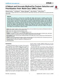
Introduction At present, plans are being made for the construction of Liquefied Natural Gas pipes in the sea bed off the coast of Hong Kong. To this end, dredging is necessary which causes plumes of silt in the water. The silt particles float in the water for a relatively long period of time, until they settle on the sea bed eventually. Unfortunately, both phenomena are harmful to coral reefs and Chinese white dolphins, two protected species that live in the sea near to Hong Kong. For this reason, before the plans can be carried out, it is necessary to determine how much of the ocean may be affected by those plumes. Water is indispensable for all organisms. People use it for drinking, fishing, bathing, irrigating, shipping, and so on. As a consequence, it is very important that its quality is maintained. The quality of water is determined by the concentrations of the substances it contains, such as oxygen, salts, silt and bacteria. From the example above it is clear that it could easily be diminished. The question is: could this be foreseen?

Figure 1.1: Forecast by Delft3D-WAQ of silt plumes near Hong Kong Fortunately, software is already available for this purpose. Delft3D-WAQ, a simulation program that has been developed by WL | Delft Hydraulics, is a useful tool in forecasting water quality. In particular, it is able to predict the size of silt plumes caused by dredging (see Figure 1.1). Basically, the software approximates the solution of the advection diffusion reaction equation by means of the finite volume method. Since it is often necessary to predict one or two years ahead, large time steps are preferred in order to have limited computing time. However, there are two aspects that need improvement. First of all, the current schemes are either

2

Introduction 35

35

30

30

25

25

20

20

15

15

10

10

5

5

0

0

(a) Accurate explicit scheme (Scheme 12, see Appendix A), computational time ≈ 176 min.

(b) Robust implicit scheme (Scheme 16, see Appendix A), computational time ≈ 9 min.

Figure 1.2: Simulation by Delft3D-WAQ of salinity in an estuary near Hong Kong. The colors of the cicles indicate measured values. explicit higher order schemes that are not robust (see Figure 1.2(a)), or implicit first order schemes that are inaccurate (see Figure 1.2(b)). Moreover, the convergence speed of the present iterative solver for linear systems is unsatisfactory for diffusion dominated problems. In other words, in this report, answers to the following question will be sought: 1. Is it possible to construct a finite volume scheme for the advection diffusion equation that is both accurate and robust? 2. Can the convergence speed of the present iterative solver for linear systems be increased for diffusion dominated problems? In other words: can the damage done to dolphins and coral reefs be estimated better and faster? The first part of this thesis, in which the numerical model is constructed, provides an answer to the first question. In Chapter 2, a physical water quality description is translated into a mathematical model that is based on the advection diffusion reaction equation. The solution to this model can be approximated by means of the finite volume method, which is discussed in Chapter 3. Chapter 4 considers accurate explicit flux correcting transport schemes. Robust theta schemes are considered in Chapter 5. In Chapter 6, the local-theta scheme is considered, which attempts to combine the advantages of the previous methods, to obtain a scheme that is both accurate and robust. A summary and recommendations can be found in Chapter 7. The second part of this thesis describes some basic theory for solving the numerical model, which forms a first step towards the answer of the second question. Implicit variants of the finite volume method require the solution of many large linear systems. In order to solve these systems efficiently, iterative solvers are considered in Chapter 8. Useful tools in improving the performance of iterative schemes are preconditioning (Chapter 9) and reordering of the matrix (Chapter 10). Chapter 11 discusses storage schemes for sparse matrices that can save both memory and time. A summary is given in chapter 12.

Part I

Constructing the numerical model

Chapter 2

Modeling water quality 2.1

Physical water quality model

The quality of water is determined by the concentrations of the substances it contains, such as oxygen, algae, salts, bacteria, viruses, toxic heavy metals, pesticides, and silt. These concentrations can be affected in two ways. Firstly, particles can be transported through the water in several ways. Moreover, water quality processes play an important role. Both phenomena will be discussed briefly below.

2.1.1

Transport

A substance can be transported by diffusion, advection, and by an own movement that is independent of the preceding types of transport.

t

t

t

tt t ttt tt t

t t t tt t t t t

t

t

t t

t

t

Figure 2.1: Molecular diffusion Molecular diffusion is the spontaneous spreading of matter due to the random movement of molecules. Figure 2.1 displays a schematic visualisation of this mixing process. Advection is the transport of a substance due to the motion of the fluid. The flow carries the particles in the downstream direction. Figure 2.2 illustrates how turbulent flow can lead to what is called turbulent mixing. Although turbulent mixing is a result of advection, it is often modeled as diffusion. For this reason, it is sometimes referred to as turbulent diffusion. Own movement is any movement that is not caused by advection or diffusion. This kind of movement could be forced by gravity, the substance itself, or the wind. Gravitational movement arises when there is a difference between the density of the substance and that of the water. Silt, for example, is heavier than water. Therefore, it will generally have an extra downward motion. Active movement only applies to organisms that can ‘swim’ in some sense. Examples are shrimps, fish, and certain algae that can propel themselves through the water. Floating movement is the

6

Modeling water quality

Figure 2.2: Turbulent mixing motion that a floating substance obtains from the wind. As a result, its concentration is generally higher on the downwind water surface side of the area.

2.1.2

Water quality processes

Apart from transport, water quality processes can have a great effect on the concentration of a substance. These processes involve the interaction between the substances. Examples are photosynthesis, mineralisation, sedimentation, nitrification, and the mortality of bacteria. For a detailed description of these processes, see e.g. [man05, Chapter 8] or [Pos05].

2.2

Mathematical water quality model

According to the physical description above, water quality is affected by transport and water quality processes. Transport due to advection and own movement can be modeled by one advection term. Adding the molecular diffusion and the water quality processes to the model, the mathematical water quality model boils down to the advection diffusion reaction equation, one for each substance that needs to be modeled. Model 2.1 (Water quality model): Consider a substance that is dissolved in flowing water. Let c(x, t) denote its (unknown) concentration, d(x, t) its molecular diffusion coefficient, and u(x, t) its velocity due to advection1 and own movement. Let p(x, t) represent all relevant water quality processes. p may also depend on c or on the concentration of other substances. For this substance, the water quality model reads:         

∂c ∂t (x, t)

+ ∇ · u(x, t)c(x, t) − d(x, t)∇c(x, t) c(x, 0) c|x∈∂D1 (∇c · n)|x∈∂D2

= = = =

p(x, t), ◦ c (x), c˘(x, t), 0.

(2.1)

◦

Here, t ∈ [0, T ] and x ∈ D ⊂ Rm (m=1,2,3). c (x) is the initial condition. The boundary of D is partitioned according to ∂D = ∂D1 ∪ ∂D2 . Here, ∂D2 is the part of the boundary through which no transport takes place (the shore) which is modeled with the help of a homogeneous Neumann boundary condition. On ∂D1 , a Dirichlet boundary condition is imposed.2 n is the outward normal unit vector on ∂D. y 1 In general the velocity due to advection is conform the velocity profile of the water. However, it is possible that a substance is not being advected, but e.g. lying on the bottom. 2 Of course, there are other types of boundary conditions, but these are not considered in this report.

2.3 Summary

2.3

7

Summary

The quality of water is determined by the concentrations of the substances it contains. These concentrations can be affected by transport and water quality processes. The corresponding mathematical model is the advection diffusion reaction equation, one for each substance that needs to be simulated.

8

Modeling water quality

Chapter 3

Finite Volume Method In general, it is impossible to obtain the analytical solution of the water quality model (Model 2.1). Fortunately, a numerical approximation can be computed by means of the finite volume method. The two main ingredients of the finite volume method are an integral form and a subdevision of the spatial domain into ‘finite volumes’. Roughly speaking, the finite volume method approximates the integral form for each of those volumes. After that, the resulting system is solved to obtain an approximation of the solution of the original model. Good references on the finite volume method are, for instance, [BO04], [God96, Chapter 4], and [Krö97, Chapter 3].

3.1

Grid

The first step towards a finite volume approximation is the subdivision of the spatial domain into smaller volumes. These volumes will be referred to as grid cells, although they need not be stacked in any regular way. In each grid cell, the average concentration of a substance is considered, which forms a good approximation for the concentration at the center of the volume. Definition 3.1 (Cell centered grid): A cell centered grid of a spatial domain D ⊂ Rd consists of a set of closed control volumes V = {Vi ⊂ D : i = 1, ..., I} and a set of storage locations X = {xi ∈ D : i = 1, ..., I} such that 1. xi is at the center of mass of Vi ; 2. the volumes cover the entire spatial domain: D=

I [

i=1

Vi ;

3. the volumes do not overlap in the sense that, for all i 6= j, either Vi ∩ Vj = ∅, or, if the volumes are adjacent, Vi ∩ Vj = ∂Vi ∩ ∂Vj , where ∂Vi denotes the boundary of Vi . The grid is denoted as G = (V, X ). In the one-dimensional case, the grid is chosen so that x1 < x2 < ... < xI . y

10

Finite Volume Method

Remark 3.2 (Grid in WAQ): WAQ often receives the velocity profile from Delft3D-FLOW, another simulation program that has been developed by WL | Delft Hydraulics. This program simulates water flow by computing an approximate solution of the shallow water equations. FLOW can handle two types of structured grids, which are both curvilinear and staggered in the horizontal direction. Figure 3.1 illustrates the different approaches in the vertical direction. The σ-grid uses a fixed number of time dependent boundary-fitted layers. The top layer fits the water surface, whereas the bottom layer fits the sea bed. A z-grid uses time-independent horizontal layers. Unlike the σ-grid, the number of (active) cells per column may vary. WAQ’s grid results from aggregating adjacent cells of the mesh that is used by FLOW. From the example in Figure 3.2 it becomes clear that this generally leads to an unstructured grid. Some schemes in WAQ require some structure though. In practice, the grid is usually strongly non-uniform. Moreover, the cells may be a thousand times as wide as they are high. y

Figure 3.1: Side view of the structured grid types of FLOW: σ-grid (left) and z-grid (right)

3.2

Integral form

The second main component of the finite volume method is an integral form of the model, which basically results from integrating the model equation. Definition 3.3 (Integral formulation of the water quality model): Consider Model 2.1. Let G = ({V1 , ..., VI }, {x1 , ..., xI }) be a (time-dependent) cell-centered grid for the (time-dependent) space domain D. If K grid cells are adjacent to the open boundary ∂D1 , introduce K adjacent virtual cells VI+1 , ..., VI+K . Let Ji contain the indices of the neighbors of grid cell Vi : Ji = {j ∈ {1, ..., I + K} : Vi ∩ Vj 6= ∅}. Let Sij denote the joint boundary of neighboring grid cells Vi and Vj : Sij = ∂Vi ∩ ∂Vj . Let nij be the unit normal vector on Sij that points in the direction of Vj . The integral form of Model 2.1 reads Z Z XZ d uc − d∇c · nij dx = (3.1) p dx. c dx + dt Vi Sij Vi j∈Ji

y

3.2 Integral form

11

Figure 3.2: An example of a grid in WAQ (bottom), resulting from the aggregation of grid cells of the grid used by FLOW (top)

12


WAQ works with average values of the velocity on the faces of the grid cells. For this reason, below, the integral form is rewritten in terms of these average velocities, by expressing the velocity as the sum of the average velocity and the deviation of this mean value. After separating these two components in the model, it is assumed that the remaining pure deviation terms can be modeled as an additional diffusion term. Proposition 3.4: Consider the integral form that was defined in Definition 3.3. Define the following boundary averages and their deviations: Z 1 cij (t) = c(x, t) dx, |Sij | Sij Z 1 uij (t) = u(x, t) dx, |Sij | Sij c˜ij (x, t) ˜ ij (x, t) u

= c(x, t) − cij , = u(x, t) − uij ,

x ∈ Sij , x ∈ Sij ,

where |Sij | denotes the surface area of Sij . Then, ∀i = 1, ..., I: Z Z Z X d ˜ ij · nij dx = p dx. |Sij |cij uij · nij − d∇c − c˜ij u c dx + dt Vi Vi Sij

(3.2)

j∈Ji

Proof. The advection term can be rewritten according to: Z Z Z cu · nij dx = cij uij · nij dx + Sij

Sij

Sij

Z

Z

+

Sij

˜ ij · nij dx + cij u

˜ ij · nij dx c˜ij u

Sij

c˜ij uij · nij dx.

Since the average deviation of the average is zero, this reduces to: Z Z Z ˜ ij · nij dx cu · nij dx = cij uij · nij dx + c˜ij u Sij

Sij

= |Sij |cij uij · nij +

Sij

Z

Sij

˜ ij · nij dx. c˜ij u

Substitution ends the proof.

1 |Sij |

R

˜ · nij dx in (3.2) can be interpreted as turbulence on a c˜ u Assumption 3.5: The term Sij ij ij sub-grid scale [Pos05, p.27]. It is assumed that this term can be modeled as an additional diffusion ˜ : D × [0, T ] → Rm×m such that (3.2) is equivalent to: term, i.e. ∃ D Z Z Z X d ˜ p dx. |Sij |cij uij · nij − (3.3) D ∇c · nij dx = c dx + dt Vi Vi Sij j∈Ji

˜. Note that the molecular diffusion coefficient d, has been included in D

y

Remark 3.6 (Magnitude of additional diffusion): The order of magnitude of the additional diffusion, that results form the assumption above, depends on size of the grid cells and on the magnitude of the velocity. Typically, WAQ uses an additional diffusion of the following order of magnitude: m 1 2 3

order of magnitude of the additional diffusion 1000 m 2 s −1 10 m 2 s −1 1 m 2 s −1

Normally, the molecular diffusion coefficient d lies between 0 m 2 s −1 and 1 m 2 s −1 , regardless of the dimension. Therefore, diffusion dominated problems mainly occur in the one- and twodimensional cases. y

3.3 Finite volume method

3.3

13

Finite volume method

The finite volume method uses separate spatial and time discretisation. First, spatial discretisation is applied to approximate the integral form in terms of cell averages and numerical fluxes. After that, the time domain is discretised to solve the resulting system of ordinary differential equations. Method 3.7 (Finite Volume Method (FVM)): The Finite volume method obtains an approximation of the solution of Model 2.1 in the following manner: 1. Approximate (3.3) by X d|Vi |ci |Sij |φij (ci , cj ) = |Vi |pi , + dt

i = 1, ..., I,

(3.4)

j∈Ji

where |Vi | denotes the volume of Vi , and ci and pi denote the following cell averages: ( R 1 i = 1, .., I, |Vi | Vi c(x, t) dx, R ci (t) = 1 t) dx, i = I + 1, .., I + K, c ˘ (x, |Vi ∩∂D1 | Vi ∩∂D1 Z 1 p(x, t) dx, pi (t) = i = 1, ..., I, |Vi | Vi and φij is a so-called numerical flux function 1 : φij (ci , cj )

≈ cij uij · nij −

1 |Sij |

Z

Sij

˜ ∇c · n dx, D ij

(3.5)

2. Discretise the time domain as follows: 0 = t0 < t1 < ... < tN ≤ T, and apply an ODE solver (see e.g. [BF01, Chapter 5]) to (3.4) to obtain a system of the form2 n−1 gin (c1n−1 , ..., cI+K , cn1 , ..., cnI+K ) = 0,

i = 1, ..., I; n = 1, ..., N.

(3.6)

Here, cni is short for ci (tn ). In the remaining of this part of the thesis, a generalisation of this convenient notation will be used, i.e. q n := q(tn ) for each quantity q(t). The solution of this system approximates the solution of the model: c(xi , tn ) ≈ cni ,

i = 1, ..., I; n = 1, ..., N.

y

Remark 3.8 (Numerical flux in WAQ): As a rule, WAQ uses a central difference approach for the diffusion term and a separate finite difference approach for the advection term. More precisely, the numerical flux function φij is of the form: φij = ψij − dij

cj − ci , kxj − xi k2

where dij = dji represents the total amount of diffusion between Vi and Vj , and ψij ≈ cij uij · nij approximates the advection term by means of a certain finite difference approach. y Remark 3.9 (Dealing with nonlinearity): Note that p may depend nonlinearly on the concentration of any substance that is included in the water quality model. In order to avoid the necessity of solving a complex nonlinear system, WAQ uses the following strategy. 1φ ij may also depend on concentrations other than ci and cj . However, such flux functions are not considered in this thesis. 2 g n may also depend on other times than t n−1 and tn . However, such time-discretisations are not considered i in this thesis.

14

Finite Volume Method 1. Suppose that cin−1 is known. Initially, leave transport out of consideration, and deal with the water quality processes in an explicit manner. In other words, compute intermediate n states ˆci by means of: n

|Vin |ˆci − |Vin−1 |cin−1 tn − tn−1

= |Vin−1 |pin−1 ,

i = 1, ..., I.

2. After that, compute cni by solving d|Vi |ci dt

= −

X

j∈Ji

|Sij |φij (ci , cj ),

i = 1, ..., I,

n with the help of an ODE solver (see e.g. Method 4.4 or Method 5.1) using ˆci instead of cin−1 .

Note that this fractional step approach introduces an error. On the other hand, it involves linear systems only, as long as the flux functions are linear. y The remainder of this part of the thesis will focus on the second step of the strategy above.

3.4

The quality of a finite volume method

The quality of a finite volume scheme is determined by a combination of accuracy and robustness. These topics are discussed briefly below.

3.4.1

Accuracy

Several properties are related to accuracy. First of all, the scheme should not conflict with the law of conservation of mass. Usually, mass conservation is a result of anti-symmetrical flux functions (φij = −φji ). Definition 3.10 (Mass conservation): Consider Method 3.7 for p = 0 (no processes) and ∂D1 = ∅ (no open boundary3 ). The scheme is mass conservative, if the total amount of mass in the interior grid cells does not change in time: PI PI n−1 n−1 n n |ci , n = 1, ..., N y i=1 |Vi |ci = i=1 |Vi Additionally, the method should yield the exact solution for infinitely small grid cells and time steps. In that case, the method is called convergent.

Definition 3.11 (Global truncation error): The global truncation error of Method 3.7 at time tn is defined as: eni = c(xi , tn ) − cni , i = 1, ..., I. y Definition 3.12 (Convergence): Consider the Method 3.7. Let the spatial mesh sizes and the time steps be decreasing functions of a parameter h. The method converges at time tn with respect to some norm k.k, if lim ken k = h↓0

0,

tn , x1 , ..., xI fixed.

Here, en is the vector containing the global truncation errors.

y

In practice, the global truncation error is (generally) not equal to zero, since the grid cells and the time steps are not infinitely small. Therefore, it is convenient to have an indication of the accuracy, which is provided below for the one-dimensional equidistant case. 3 In

case of an open boundary, the change in mass should match the transport through the open boundary.

3.4 The quality of a finite volume method

15

Definition 3.13 (Order of accuracy): Consider the one-dimensional variant (m = 1) of Method 3.7 with constant time step ∆t and constant cell width ∆x. The method is said to be s1 order accurate in time and s2 order accurate in space with respect to some norm k.k, if ken k

= O(∆ts1 ) + O(∆xs2 ).

Here, en is the vector containing the global truncation errors.

y

Intuitively, convergence can only occur if the local truncation error is small enough. This condition is called consistency. Definition 3.14 (Local truncation error): The local truncation error of Method 3.7 at time tn is defined as: eñi = gin c(x1 , tn−1 ), ..., c(xI+K , tn−1 ), c(x1 , tn ), ..., c(xI+K , tn ) , i = 1, ..., I. y

Definition 3.15 (Consistency): Consider Method 3.7. Let the spatial mesh sizes and the time steps be decreasing functions of a parameter h. The method is consistent at time tn with respect to some norm k.k, if lim k˜ en k = h↓0

0,

tn , x1 , ..., xI fixed.

ñ is the vector containing the local truncation errors. Here, e

3.4.2

y

Robustness

Next to accuracy, efficiency is of great importance. A method is said to be robust if its “efficiency is insensitive to changes in the problem, such as variations in grid point distribution (especially cell aspect ratios)” [Wes01, p. 263], or in the velocity profile. The robustness of a scheme is usually related to conditions that ensure stability, positivity, and non-oscillatory behavior. This section discusses these properties. Roughly speaking, stability means that a small perturbation of the initial condition should not lead to a completely different solution. A definition of absolute stability is given below. For more information about stability-related topics, see e.g. [Wes01, Chapter 5]. Definition 3.16 (Absolute stability): Method 3.7 is called absolutely stable with respect to some norm k.k, if there exist constants k, τ > 0 (τ may depend on the spatial mesh size) such that, if tn − tn−1 ≤ τ,

∀n = 1, ..., N,

then, for any perturbation w0 of the initial condition c0 that yields a perturbation wn of cn , kwn k ≤ kkw0 k,

∀n = 1, ..., N.

y

Next to stability, positivity is a favorable feature, because negative concentrations are unphysical. Positivity preserving schemes guarantee positive results, provided that the initial and boundary conditions are positive. Definition 3.17 (Positivity preservation): Method 3.7 (for p = 0) is positivity preserving, if c0i cni

≥ 0, ≥ 0,

i = 1, ..., I, i = I + 1, ..., I + K; n = 0, ..., N,

implies that cni ≥ 0,

i = 1, .., I; n = 1, ..., N.

y

16


Finally, the method should not generate spurious oscillations. In the one-dimensional case, the occurrence of wiggles is unlikely if the scheme is monotonicity-preserving [Wes01, p. 340]. Definition 3.18 (Monotonicity preservation): Consider Method 3.7 for p = 0 and m = 1. The scheme is monotonicity preserving, if, for every non-decreasing (non-increasing) initial condition {c0i }, the numerical solution at all later instants cni (n = 1, 2, ..., N ) is non-decreasing (non-increasing). In the multi-dimensional unstructured case, the concept of local extremum diminishing schemes is useful, which was introduced by Jameson [Jam93]. Definition 3.19 (Local Extremum Diminishing (LED)): Consider Method 3.7 for p = 0. The system of ODEs that results from the spatial discretisation is called local extremum diminishing, if a local maximum cannot increase and a local minimum cannot decrease. y Observe that a LED scheme is automatically positivity preserving and L∞ -stable, as the global maximum cannot increase and the global minimum cannot decrease [KT02, p. 531]. However, the nice features of a LED spatial discretisation may still get disturbed by time discretisation. For this purpose, a local and a global discrete maximum principle will be discussed now. The local discrete maximum principle basically states that each concentration cni lies between the minimum and maximum of the concentrations that it depends on. The global discrete maximum principle implies that each concentration cni lies between the minimum and the maximum of the initial and the boundary conditions. Definition 3.20 (Local discrete maximum principle): Consider Method 3.7 for p = 0. Suppose a scheme of the form: X X anii cni + anij cnj = bnij cjn−1 , i = 1, .., I, anij 6= 0 (j ∈ Ani ∪ {i}), bnij 6= 0 (j ∈ Bin ), j∈An i

j∈Bin

where Ai ⊂ Ji and Bi ⊂ Ji ∪ {i}. The scheme admits a local discrete maximum principle, if, for any solution to the scheme, either cni = cnj = ckn−1 ,

j ∈ Ani , k ∈ Bin ,

(3.7)

or min

minn cnj , minn cjn−1

j∈Ai

j∈Bi

< cni < max

for all i = 1, ..., I and for all n = 1, .., N .

maxn cnj , maxn cjn−1 ,

j∈Ai

j∈Bi

(3.8) y

Definition 3.21 (Global discrete maximum principle): Consider Method 3.7 for p = 0. Suppose a scheme of the form: X X anij cnj = bnij cjn−1 , anii cni + i = 1, .., I, anij 6= 0 (j ∈ Ani ∪ {i}), bnij 6= 0 (j ∈ Bin ), j∈An i

j∈Bin

where Ai ⊂ Ji and Bi ⊂ Ji ∪ {i}. The scheme satisfies the global discrete maximum principle, if, for any solution to the scheme, for each i = 1, ..., I and for each n = 1, ..., N , there is a non-decreasing path to the boundary or to to the initial condition in the sense that there exist j1 , j2 , ..., jE ∈ {1, ..., I + K} and m1 , m2 , ..., mE ∈ {0, 1, ..., N } such that me e • je+1 ∈ Am je ∪ Bje ,

• me+1 ≤ me , • either mE = 0 or jE ∈ {I + 1, ..., I + K}, mE 1 • cni ≤ cm j1 ≤ ... ≤ cjE ,

3.5 Summary

17

and if, similarly, a non-increasing path exists. As a consequence, the scheme satisfies:         max {c0j }, min {c0j }, min {cnj }, ≤ cni ≤ max max {cni } , min j=I+1,...,I+K j=I+1,...,I+K  j=1,...,I  j=1,...,I n=0,...,N n=0,...,N | | {z } {z } =:m

(3.9)

=:M

for all i = 1, ..., I + K and for all n = 0, ..., N .

y

Often, the global discrete maximum can be derived by successive application of the local discrete maximum principle. For the fully explicit case it is mentioned in [BO04, p. 13] that the local discrete maximum principle “precludes spurious extrema and O(1) Gibbs-like phenomena”. In the general implicit case, the global discrete maximum principle implies that, for each concentration cni , it is possible to step through the stencil, passing only concentrations that are not larger than cni , until either a boundary cell (i = I + 1, ..., I + K) or an initial cell (n = 0) is reached. A similar result holds for non-increasing values. In other words: a local maximum in the interior can only be the result of the transportation of a local maximum in the initial or boundary conditions and, in that sense, can not be spurious. In the remaining of this thesis this will be called non-oscillatory behavior. Another convenient consequence of the global discrete maximum principle is that the scheme is positivity preserving and absolutely stable with respect to k.k∞ . Theorem 3.22: If Method 3.7 satisfies the global discrete maximum principle (3.9), then the scheme is positivity preserving. Proof. Trivial.

Theorem 3.23: If Method 3.7 satisfies the global discrete maximum principle (3.9), then the scheme is absolutely stable with respect to k.k∞ . Proof. (See also [Wes01, p. 170-171].) Let w0 be a perturbation of the initial condition c0 that yields a perturbation wn of cn . As both cn and cn + wn satisfy the (linear) scheme, subtraction yields that wn also satisfies the scheme. Applying the global maximum principle (3.9), it follows that min{wj0 } ≤ win ≤ min{wj0 } j

j

Hence, kwn k∞ ≤ kw0 k∞ , As a result, the scheme is absolutely stable with respect to k.k∞ (see also Definition 3.16 for k = 1).

3.5

Summary

The solution of the water quality model can be approximated by means of the finite volume method (FVM). The grid that is used by Delft3D-WAQ is usually three-dimensional, unstructured, and strongly non-uniform. Water quality processes are treated in an explicit manner, in order to avoid the necessity of solving a nonlinear system. The quality of a finite volume scheme is determined by accuracy and robustness. In this respect, the local and the global discrete maximum principle are favorable properties of a FVM because they imply stability, positivity and non-oscillatory behavior.

18


Chapter 4

Accurate explicit schemes In the introduction it was mentioned that WAQ’s current schemes are either explicit higher order schemes that are not robust, or implicit first order schemes that are inaccurate. This chapter considers the first category.

4.1

Local extremum diminishing flux functions

The flux function that is used in a finite volume scheme determines much of the characteristics of the scheme. The beauty of first order upwind discretisation (4.1) is that it leads to a linear local extremum diminishing (LED) system of ODEs. This is easy to prove with the help of the following theorem. Theorem 4.1: Consider Method 3.7 for p = 0. Suppose that spatial discretisation has resulted in a system of the form: X d|Vi |ci |Sij |φij = − dt j∈Ji X −|Sij |φij = −γji ci + γij cj , (−γji + γij ) = 0. j∈Ji

If γij ≥ 0 for all i and j, then, the system is LED. Proof. (See also [Jam93, p. 385] or [KT02, p. 531].) Suppose that ci is a local maximum. So ci ≥ cj for all j ∈ Ai . Consequently: d|Vi |ci dt

=

X

(−γji ci + γij cj )

j∈Ji

=

X

j∈Ji

=

X

−γji ci +

X

j∈Ji

γij (cj − ci ) +

(−γji + γij ) ci +

j∈Ji

|

X

j∈Ji

{z

=0

}

X

γij ci

j∈Ji

γij (cj − ci ) ≤ 0. |{z} | {z } ≥0

≤0

Therefore, the local maximum can not increase. Similarly, it can be shown that a local minimum can not decrease. Hence, the scheme is LED. Proposition 4.2: Consider Method 3.7 for p = 0, after applying first order upwind spatial discretisation to the advection terms and central difference discretisation to the diffusion terms: X d|Vi |ci |Sij |φij , = − dt j∈Ji

20

Accurate explicit schemes

where φij is the following flux function: − |Sij |φij

= −γji ci + γij cj = −|Sij | min{0, uij · nij } −

γij

If the velocity profile is conservative in the sense that X |Sij |uij · nij =

(4.1) dij kxj − xi k2

.

0,

(4.2)

j∈Ji

then, the resulting system is LED. Proof. First, note that γij ≥ 0. Furthermore, observe that X X |Sij | − max{0, uji · nji } + max{0, uij · nij } (−γji + γij ) = − j∈Ji

j∈Ji

=

= (4.2)

=

−

−

X

j∈Ji

X

j∈Ji

|Sij | min{0, uij · nij } + max{0, uij · nij }

|Sij |uij · nij

0

Applying Theorem 4.1 yields that the scheme is LED.

A similar argument does not hold for central discretisation (4.3), which is of second order. However, the proposition below shows how central discretisation can be rendered LED by eliminating negative coefficients by adding artificial diffusion. This strategy results in what will be called upwinded central discretisation. Proposition 4.3: Consider Method 3.7 for p = 0. Apply central discretisation to the advection terms and the central difference scheme to the diffusion terms to obtain: d|Vi |ci dt

= −

X

j∈Ji

|Sij |φ˜ij ,

where φ˜ij is the following flux function: − |Sij |φ˜ij γ˜ij

= −˜ γji ci + γ˜ij cj uij · nij dij − . = −|Sij | 2 kxj − xi k2

(4.3)

If φij is the following ‘upwinded’ version of φ˜ij : − |Sij |φij γij

= −γji ci + γij cj = γ˜ij + max{0, −˜ γij , −˜ γji },

and if the velocity profile is conservative in the sense that X |Sij |uij · nij = 0, j∈Ji

then, the system d|Vi |ci dt

= −

X

j∈Ji

|Sij |φij ,

(4.4)

(4.5)

4.2 Explicit schemes

21

is LED. Proof. First, note that γij ≥ 0. Furthermore, observe that X X (−˜ γji + γ˜ij ) (−γji + γij ) = j∈Ji

j∈Ji

=

−

(4.5)

=

X

j∈Ji

|Sij |uij · nij

0

Applying Theorem 4.1 yields that the scheme is LED.

According to Kuzmin et al. [KMT, p. 4-5], who proposed this strategy, the physical diffusion is “automatically detected and the amount of artificial diffusion is reduced accordingly.” For diffusion dominated problems, upwinded central discretisation is identical to central discretisation, “since the coefficients are nonnegative from the outset”. For the one-dimensional advection equation, upwinded central discretisation is equivalent to first order upwind discretisation.

4.2

Explicit schemes

Method 4.4 (Explicit (upwind) scheme): The explicit scheme is a FVM (Method 3.7) that reads (for p=0): |Vin |cni − |Vin−1 |cin−1 tn − tn−1

= −

X

j∈Ji

n−1 n−1 |Sij |φij ,

where φij is a flux function. If φij is as in (4.1), the scheme is known as the explicit upwind scheme. y Figure 4.1 displays the results of the explicit upwind scheme for the following test case. Test case 4.5 (One-dimensional advection equation): This test case is the one-dimensional advection equation with periodic boundary conditions:  ∂c ∂c = 0, x ∈ [0, 10], t ≥ 0,  ∂t + u ∂x c(x, 0) = 1[2,4] (x) 21 1 − cos(πx) + 1[6,8] (x), x ∈ [0, 10],  c(0, t) = c(10, t), t ≥ 0. Note that the (exact) solution is periodic with a period of 10.

y

For this test case, the explicit upwind scheme reads: ∆xi cni − ∆xi cin−1 ∆t

n−1 , = −ucin−1 + uci−1

(4.6)

where ∆t = tn − tn−1 is the constant time step and ∆xi = |Vin−1 | = |Vin | is the cell width. The scheme will be stable, positivity preserving and non-oscillatory if ∆xi ≤ 1, u∆t

i = 1, ..., I,

(4.7)

which results from (5.2) for θ = 0. This condition is also known as the Courant-Friedrichs-Lewy (CFL) condition [LeV02, Section 4.4]. Note that the smallest grid cell is responsible for the number of time steps. This explains why the number of time steps N is much larger in Figures 4.1(c) and 4.1(d) than in Figures 4.1(a) and 4.1(b). Apparently, the scheme is not robust. Furthermore, the explicit upwind scheme is not very accurate for this test case. The numerical solution is smeared out compared to the exact solution. Observe that this effect is larger in Figures 4.1(c) and 4.1(d)

22

Accurate explicit schemes u=1, I=100, T=10

u=1, I=100, T=50

1.5

1.5

1

exact solution Explicit upwind (N=551)

c (concentration)

c (concentration)


0.5

0 0

1

0.5

0 2

4

6

8

10

0

2

4

x

6

(a) equidistant grid, 1 period u=1, I=120, T=10

u=1, I=120, T=50 1.5


1


c (concentration)

c (concentration)

10

(b) equidistant grid, 5 periods

1.5

0.5

0 0

8

x

1

0.5

0 2

4

6

8

10

0

2

x

4

6

8

10

x

(c) non-equidistant grid, 1 period

(d) non-equidistant grid, 5 periods

Figure 4.1: Explicit upwind scheme (Method 4.4) for Test case 4.5

than in Figures 4.1(a) and 4.1(b). This is explained by the fact that, for a one-dimensional equidistant grid, the explicit upwind scheme introduces the following additional artificial diffusion coefficient: u∆x 2

u∆t 1− ∆x

.

(4.8)

This follows from Proposition 5.2 for θ = 0. A simple calculation shows that the numerical diffusion in Figures 4.1(a) and 4.1(b) reads 0.0198, whereas it is equal to 0.1818 (in the largest cells) in Figures 4.1(c) and 4.1(d). The next section discusses a strategy to diminish this numerical diffusion.

4.3

Flux corrected transport

Theorem 4.6 (Godunov’s barrier theorem): Consider the one-dimensional advection equation (Model 2.1 for m = 1, d = 0, p = 0, and u constant): ∂c ∂c +u ∂t ∂x

=

0.

4.3 Flux corrected transport

23

Suppose that the model is solved by means of Method 3.7 with a constant mesh width ∆x and a constant time step ∆t. Assume that the scheme can be written in the form: X n−1 cni = . γj ci+j j

If the scheme is second-order in the sense that the exact solution is reproduced if the initial condition is a polynomial of second degree, then, the scheme cannot be monotonicity preserving, unless |u|∆t ∆x ∈ N. Proof. See [Wes01, Theorem 9.2.2].

Roughly speaking, Godunov’s barrier theorem implies that a linear method either is relatively inaccurate (remember the artificial diffusion of the explicit upwind scheme), or it has a tendency to generate spurious oscillations [BO04, p.19]. The Flux Correcting Transport (FCT) algorithm attempts to combine a non-oscillatory first order flux function with an accurate higher order flux function by means of a nonlinear limiter. Roughly speaking, the algorithm uses a convex combination of the two flux functions, instead of just one of them. This strategy can also be described as updating the first order flux with a limited correction flux. Method 4.7 (Explicit FCT scheme): The explicit FCT scheme is a FVM (Method 3.7) of the following form (for p = 0): |Vin |cni − |Vin−1 |cin−1 tn − tn−1

= −

X

j∈Ji

n−1 n−1 n−1 n ñ−1 |Sij | φîj . φij − φîj + lij

(4.9)

Here, φîj is a non-oscillatory first order numerical flux function of the form (3.5), and φ˜ij is a higher order one. The difference φ˜ij − φîj can be interpreted as a correction term, which is limited y by lij . If φîj is as in (4.1), the explicit upwind FCT scheme is obtained. n Note that choosing lij = 0 corresponds to applying the first order method. On the other hand, n setting lij = 1 is equivalent to using the higher order method. The limiter that is used by scheme 12 of WAQ is a generalised version of the one-dimensional limiter that was proposed by Boris & Book [BB73], the founders of the FCT algorithm. This limiter has been extended to the multidimensional case on a structured grid by Zalesak [Zal79]. Below, it is further generalised for an unstructured grid. The limiter allows as much correction as possible, provided that it generates no new local extrema.

Method 4.8 (Explicit FCT scheme ` a la Boris & Book): This method results from the explicit FCT scheme (Method 4.7) by using the following limiter: 1. Suppose that cin−1 is known from the previous time step. Compute a first order approximan n = 0, which is equivalent to applying the explicit scheme tion ˆci by means of (4.9) with lij (Method 4.4) with the lower order flux function φîj : n

n−1

|Vin |ˆci − |Vin−1 |ˆci tn − tn−1

= −

X

j∈Ji

n−1 ˆn−1 |Sij |φij .

2. Define the flux correction ∆φnij as follows: ∆φnij

n−1 n−1 = φ˜ij − φîj

3. Since ∆φnij often corrects the numerical diffusion of the first order flux, it is sometimes referred to as anti-diffusion. Because an anti-diffusion term should not behave as a diffusion term, put ∆φnij = 0 if n n ∆φnij (ˆci − ˆcj ) > 0.

24

Accurate explicit schemes If this prelimiting step is not performed, the flux correction may smooth the low-order solution, or it may cause small-scale numerical ripples [KT02, p.541]. Since it is unphysical for an anti-diffusion term to be directed from a higher concentration to a lower concentration, the effect of the adjustment above is minimal in practice [Zal79, p. 342]. n

4. Construct an upper and a lower bound for cni by means of the first order approximation ˆci : cmax i

=

cmin i

=

n max {ˆcj },

j∈Ji ∪{i}

n min {ˆcj }.

j∈Ji ∪{i}

5. The amount of mass that flows into cell Vi as a result of the flux correction (without the limiter) reads: X n (tn − tn−1 )|Sij | max{0, − ∆φnij }. = λ+ i j∈Ji

The allowed mass increase is, however: µ+ i

n − ˆci . = |Vi | cmax i

Thus, the fraction of mass that is allowed to flow into the cell is given by:  n o min 1, µ+ i , λ+ i > 0, λ+ i νi+ = 0, λ+ i = 0, Introduce analogue quantities for mass decrease: X n λ− (tn − tn−1 )|Sij | max{0, ∆φnij }, = i j∈Ji

µ− i νi−

n , = |Vi | ˆci − cmin i  n −o min 1, µi , λ− > 0, i λ− i = 0, λ− i = 0.

6. The limiter is the mass fraction that is allowed by both adjacent cells: ( min{νj+ , νi− }, ∆φnij ≥ 0, n lij = min{νi+ , νj− }, ∆φnij < 0. y Remark 4.9: Alternatively, next to the first order approximation mation cin−1 could be used to determine the bounds cmax and cmin : i i n o n max{cjn−1 , ˆcj } , cmax = max i j∈Ji ∪{i} o n n min ci = min min{cjn−1 , ˆcj } .

ˆcni ,

the previous solution esti-

j∈Ji ∪{i}

In general, this leads to a larger limiter, which means that more flux correction is applied that diminishes numerical diffusion. However, this choice is less safe because the birth of new local extremes is no longer excluded (see also [Zal79, p. 342]). y


25

u=1, I=100, T=10

u=1, I=100, T=50

1.5

1.5 Exact solution Explicit upwind (N=551) Explicit upwind FCT (N=551)

1

c (concentration)

c (concentration)

Exact solution Explicit upwind (N=111) Explicit upwind FCT (N=111)

0.5

0

1

0.5

0

0

2

4

6

8

10

0

2

4

x


10

u=1, I=120, T=50 1.5

Exact solution Explicit upwind (N=1101) Explicit upwind FCT (N=1101) 1

Exact solution Explicit upwind (N=5501) Explicit upwind FCT (N=5501) c (concentration)

c (concentration)

8


1.5

0.5

0 0

6 x

1

0.5

0 2

4

6

8

10

x

0

2

4

6

8

10

x



Figure 4.2: Explicit upwind FCT scheme (Method 4.8) with central flux correction (4.3) for Test case 4.5

Remark 4.10 (TVD limiters): After Boris and Book proposed the FCT algorithm, many alternative limiting strategies have been developed. A popular class is formed by the Total Variation Diminishing (TVD) limiters, which includes minmod, Van Leer, MC, and superbee. These limiters y are considered for multi-dimensional unstructured grids in [KT, Sections 2 and 10]. Figure 4.2 displays the results of the explicit upwind FCT scheme (Method 4.8) with central flux correction (4.3). Compared to the explicit upwind scheme, the numerical diffusion has been reduced drastically. However, the anti-diffusion is too large in some portions of the domain, especially in Figures 4.2(a) and 4.2(b). This is explained by the fact that, for a one-dimensional equidistant grid, the explicit scheme with central fluxes introduces the following additional artificial diffusion coefficient: 1 − u2 ∆t. 2 This follows from Proposition 5.6 for θ = 0. Because negative diffusion is unphysical, central fluxes are unsuitable to serve as flux correction in the explicit FCT scheme. An alternative flux correction is provided by the Lax-Wendroff scheme. Method 4.11 (Lax-Wendroff scheme): The Lax-Wendroff scheme is a fully discrete FVM (see

26


˜ = 0): Method 3.7 for notational aspects) of the following form (for p = 0 and D |Vin |cni − |Vin−1 |cin−1 tn − tn−1

= −

X

j∈Ji

n−1 n−1 |Sij |φij ,

where n−1 φij

n−1 + = φîj

n−1 ∆ξij

kxjn−1

−

−

xin−1 k2

n−1 n−1 uij · nij (tn − tn−1 )

2kxjn−1

−

xin−1 k2

n−1 Here, φîj is the first order upwind flux: n−1 φîj

=

!

n−1 n−1 cjn−1 − cin−1 . · nij uij

n−1 n−1 n−1 n−1 max{uij · nij , 0}cin−1 + min{uij · nij , 0}cjn−1 ,

n−1 n−1 n−1 and ∆ξij is the distance1 between xin−1 and Sij · nn−1 , if uij ≥ 0, and minus the distance ij n−1 n−1 n−1 n−1 and Sij , if uij · nij < 0. between xj

Derivation. First, reduce the model to the one-dimensional advection equation with constant velocity u > 0, constant cell width ∆x > 0, and constant time step ∆t > 0. Consider the following Taylor expansion around t = tn−1 : c(x, tn )

≈ c(x, tn−1 ) + ∆t

∆t2 ∂ 2 c ∂c (x, tn−1 ). (x, tn−1 ) + ∂t 2 ∂t2

This expression can be rewritten to obtain: c(x, tn ) − c(x, tn−1 ) ∆t

∂c ∆t ∂ 2 c (x, tn−1 ) + (x, tn−1 ). ∂t 2 ∂t2

≈

Note that: ∂c ∂t ∂2c ∂t2

∂c , ∂x 2 ∂ c = u2 2 . ∂x

= −u

Hence: c(x, tn ) − c(x, tn−1 ) ∆t Applying central differences yields: cni − cin−1 ∆t

= −u

= −u

∂c ∆t 2 ∂ 2 c (x, tn−1 ). (x, tn−1 ) + u ∂x 2 ∂x2

n−1 n−1 n−1 n−1 n−1 − ci−1 + ci+1 ci+1 ∆t 2 ci−1 − 2ci . + u 2∆x 2 ∆x2

Rewriting gives: ∆x

cni − cin−1 ∆t

n−1 = −ucin−1 + uci−1 1 u∆t u∆t 1 n−1 n−1 − cin−1 ) − − cin−1 ). 1− u(ci+1 1− u(ci−1 − 2 ∆x 2 ∆x

Finally, the derivation of the generalisation to non-equidistant grids can be found in [LeV02, Section 6.17]. Figure 4.3 displays the results of the explicit upwind FCT scheme (Method 4.8) with Lax-Wendroff flux correction (Method 4.11) for Test case 4.5. Again, compared to the explicit upwind scheme, the numerical diffusion has been reduced. Where the central scheme caused too much anti-diffusion (see Figure 4.2), the Lax-Wendroff scheme seems to add a more appropriate amount. Proposition 5.7 (for θ = 0) shows that, on a one-dimensional equidistant grid, the numerical diffusion of the Lax-Wendroff scheme is equal to zero. Scheme 12 of WAQ uses Lax-Wendroff flux correction. 1 Of course, there is more than one way to define this distance. In WAQ, the distance between x and S ij is an i n is the point where the line through x and x intersects S . approximation of kxi − yij k2 . Here yij ij i j

4.4 Summary

27 u=1, I=100, T=10

u=1, I=100, T=50

1.5

1.5

1


c (concentration)

Exact solution Explicit upwind (N=111) Explicit upwind FCT (N=111)

0.5

0 0

1

0.5

0 2

4

6

8

10

0

2

4

x


10

u=1, I=120, T=50 1.5

Exact solution Explicit upwind (N=1101) Explicit upwind FCT (N=1101) 1


c (concentration)

8


1.5

0.5

0 0

6 x

1

0.5

0 2

4

6

8

x


10

0

2

4

6

8

10

x


Figure 4.3: Explicit upwind FCT scheme (Method 4.8) with Lax-Wendroff flux correction (Method 4.11) for Test case 4.5

4.4

Summary

The explicit upwind scheme is neither robust nor accurate. The former is caused by the fact that the time step is limited to ensure stability, positivity and non-oscillatory behavior. The inaccuracy is a a result of numerical diffusion, which can be diminished by means of the flux corrected transport (FCT) algorithm. Central flux correction leads to an anti-diffusion error. For this reason, the Lax-Wendroff scheme is more suitable to serve as flux corrector, as its numerical diffusion is equal to zero. Although the accuracy of the explicit FCT scheme is generally high, the robustness of the explicit scheme remains unchanged, which can result in long computational times. Scheme 12 of WAQ is an explicit FCT scheme with Lax-Wendroff flux correction.

28


Chapter 5

Robust implicit theta schemes In the introduction it was mentioned that WAQ’s current schemes are either explicit higher order schemes that are not robust, or implicit first order schemes that are inaccurate. This chapter considers the second category.

5.1

Theta scheme

Method 5.1 (Theta (upwind) scheme): The theta scheme is a FVM (Method 3.7) that reads (for p=0): |Vin |cni − |Vin−1 |cin−1 tn − tn−1

= −

X

j∈Ji

n−1 n−1 n n (1 − θ)|Sij |φij + θ|Sij |φij ,

where φij is a flux function. If φij is as in (4.1), the scheme theta upwind scheme is obtained. y u=1, I=120, T=10

u=1, I=120, T=50 1.5

exact solution Theta upwind (θ=0, N=1101) Theta upwind (θ=0.89, N=111) Theta upwind (θ=1, N=111)

1

c (concentration)

c (concentration)

1.5

0.5

0 0

exact solution Theta upwind (θ=0, N=5501) Theta upwind (θ=0.89, N=551) Theta upwind (θ=1, N=551)

1

0.5

0 2

4

6 x

(a) 1 period

8

10

0

2

4

6

8

10

x

(b) 5 periods

Figure 5.1: Theta upwind scheme (5.1) for Test case 4.5 Figure 5.1 displays the results of the theta upwind scheme for Test case 4.5. For this test case, the theta upwind scheme reads: ∆xi cni − ∆xi cin−1 ∆t

n−1 = −(1 − θ)u(cin−1 − ci−1 ) − θu(cni − cni−1 ),

(5.1)

30

Robust implicit theta schemes

where ∆t = tn − tn−1 is the constant time step and ∆xi = |Vin−1 | = |Vin | is the cell width. The scheme will be stable, positivity preserving and non-oscillatory if θ ≥1−

∆xi , u∆t

i = 1, ..., I,

(5.2)

which follows from (6.10) for constant θ. The test was performed for three different pairs of θ and ∆t that satisfy (5.2). In the fully explicit case (θ = 0, blue), this has resulted in a relatively large number of time steps. In the fully implicit case (θ = 1, red), any number of time steps is allowed, because (5.2) is unconditionally satisfied. This is the value that is used by scheme 16 of WAQ. Finally, observe that the numerical solution is more smeared out in comparison with the exact solution as θ becomes larger. In the following proposition, an expression for the numerical diffusion coefficient is derived with the help of the modified equation. Proposition 5.2: Consider the theta upwind scheme (Method 5.1) for the one-dimensional advection equation with constant velocity u > 0, constant cell width ∆x > 0, and constant time step ∆t > 0: n+1

c − cni cn+1 i + θu i ∆t

− cn+1 cn − cni−1 i−1 + (1 − θ)u i ∆x ∆x

=

0.

Let η(x, t) be a ‘sufficiently differentiable’function such that η(xi , tn ) = cni . Then, the corresponding modified equation reads ∂η u∆x ∂η (xi , tn ) + u (xi , tn ) ≈ ∂t ∂x 2 |

u∆t ∂ 2 η 1 − (1 − 2θ) (xi , tn ). ∆x ∂x2 {z }

Numerical diffusion coefficient

Proof. Because η(xi , tn ) = cni , η(xi , tn+1 ) − η(xi , tn ) ∆t η(xi , tn+1 ) − η(xi−1 , tn+1 ) +θu ∆x η(xi , tn ) − η(xi−1 , tn ) +(1 − θ)u ∆x

=

0.

Using a Taylor expansion of η around tn results in (higher order terms that will be neglected later are colored): ∆t2 ∂ 3 η ∂η ∆t ∂ 2 η (xi , tn ) + (xi , τ1 ) (xi , tn ) + 2 ∂t 2 ∂t 6 ∂t3 2 3 ∆t2 ∂ η ∆t3 ∂ η η(xi , tn ) + ∆t ∂η ∂t (xi , tn ) + 2 ∂t2 (xi , tn ) + 6 ∂t3 (xi , τ2 ) +θu ∆x 2 3 3 ∂η ∆t2 ∂ η η(xi−1 , tn ) + ∆t ∂t (xi−1 , tn ) + 2 ∂t2 (xi−1 , tn ) + ∆t6 ∂∂t3η (xi−1 , τ3 ) − ∆x η(xi , tn ) − η(xi−1 , tn ) = +(1 − θ)u ∆x

0,

5.1 Theta scheme

31

for certain τ1 , τ2 , τ3 ∈ [tn , tn+1 ]. Using a Taylor expansion of η around xi yields: ∂η ∆t2 ∂ 3 η ∆t ∂ 2 η (x , t ) + (xi , τ1 ) (xi , tn ) + i n 2 ∂t2 6 ∂t3 ∂t ∆x2 ∂ 3 η ∂η ∆x ∂ 2 η +θu (xi , tn ) + (ξ1 , tn ) (xi , tn ) − 2 ∂x 2 ∂x 6 ∂x3 ∂ ∂η ∆t∆x ∂ 2 ∂η +∆t (xi , tn ) − (ξ2 , tn ) ∂x ∂t 2 ∂x2 ∂t ∆t3 ∂ 3 η ∆t3 ∂ 3 η + (xi , τ2 ) − (ξ3 , τ3 ) 6∆x ∂t3 6∆x ∂t3 ∆x2 ∂ 3 η ∆x ∂ 2 η ∂η (xi , tn ) − (xi , tn ) + (ξ4 , tn ) +(1 − θ)u ∂x 2 ∂x2 6 ∂x3

=

0,

for certain ξ1 , ξ2 , ξ3 , ξ4 ∈ [xi−1 , xi ]. Rewriting gives: ∂η ∂η (xi , tn ) + u (xi , tn ) = ∂t ∂x

u∆x ∂ 2 η (xi , tn ) 2 ∂x2 2 ∆t ∂ η ∂ ∂η − (xi , tn ) − θu∆t (xi , tn ) 2 2 ∂t ∂x ∂t ∆t2 ∂ 3 η (xi , τ1 ) − 6 ∂t3 ∆t∆x ∂ 2 ∂η ∆x2 ∂ 3 η (ξ , t ) − (ξ2 , tn ) −θu 1 n 6 ∂x3 2 ∂x2 ∂t ∆t3 ∂ 3 η ∆t3 ∂ 3 η (x , τ ) − (ξ3 , τ3 ) + i 2 6∆x ∂t3 6∆x ∂t3 ∆x2 ∂ 3 η −(1 − θ)u (ξ4 , tn ). 6 ∂x3

Note that ∂η ∂η (xi , tn ) = −u (xi , tn ) + O(∆t) + O(∆x) ∂t ∂x 2 ∂ η ∂2η 2 (x , t ) = u (xi , tn ) + O(∆t) + O(∆x). i n ∂t2 ∂x2 Substitution yields: ∂η ∂η (xi , tn ) + u (xi , tn ) = ∂t ∂x

u∆x ∂ 2 η (xi , tn ) 2 ∂x2 ∂2η u2 ∆t ∂ 2 η 2 (x , t ) + θu ∆t (xi , tn ) − i n 2 2 ∂x ∂x2 +O ∆t2 + O ∆x2 + O(∆x∆t).

Rewriting and neglecting second order terms ends the proof.

The proposition above implies that, on an equidistant grid, the numerical diffusion coefficient of Test case 4.5 reads: u∆t u∆x 1 − (1 − 2θ) . (5.3) 2 ∆x This is illustrated in Figure 5.2 by means of a contour plot of 1 − (1 − 2θ) u∆t ∆x as a function of the CFL-number u∆t . The magenta line indicates the border of the region where the numerical ∆x diffusion is nonnegative: ∆x 1 1− . (5.4) θ≥ 2 u∆t

32

Robust implicit theta schemes 4 4 3.5 3

3

2

u∆ t/∆ x

2.5

1

2

0

1.5 1

−1

0.5

−2

0 0

0.2

0.4

θ

0.6

0.8

1

−3

Figure 5.2: Contour plot of 1 − (1 − 2θ) u∆t ∆x , the scaled numerical diffusion coefficient (5.3); the magenta border corresponds to (5.4), the (dark) purple border corresponds to (5.2) The (dark) purple line indicates the border of the region where (5.2) is satisfied. Apparently, if (5.2) is satisfied, which implies stable, positive, and non-oscillatory behavior, the numerical diffusion coefficient must be strictly positive (unless θ = 0 and u∆t ∆x = 1). At the same time, a strictly positive numerical diffusion coefficient causes artificial smearing of the solution (see Figure 5.1). Observe that the numerical diffusion grows with θ. Altogether, it is best to satisfy (5.2) with the smallest possible θ.

5.2

Theta FCT scheme

Section 4.3 described the explicit FCT scheme (Method 4.7), which is accurate, but not robust due to a severe stability criterion for the time step. The question is: will an implicit variant of such a scheme lead to a method that is both accurate and robust? For this purpose, the explicit FCT scheme will be generalized to the theta FCT scheme. Method 5.3 (Theta (upwind) FCT scheme): The theta FCT scheme is a FVM (Method 3.7) of the following form (for p = 0): X |Vin |cni − |Vin−1 |cin−1 n,n−1 ñ−1 n−1 n−1 n |Sij | (1 − θ) φîj + lij φij − φîj = − tn − tn−1 j∈Ji n,n ñ (5.5) +θ φˆnij + lij φij − φˆnij

Again, φîj is a non-oscillatory first order numerical flux function of the form (3.5), and φ˜ij is a higher order one. The difference φ˜ij − φîj can be interpreted as a correction term, which is limited by lij . If φîj is as in (4.1), the theta upwind FCT scheme is obtained. y

Note that, if θ = 0, the method corresponds to the explicit FCT scheme (Method 4.7). In the implicit case (θ > 0), Method 5.3 requires the solution of a nonlinear system, if the limiter depends nonlinearly on the concentration at the new time tn . The latter is usually the case because of Godunov’s barrier theorem (Theorem 4.6). The following method avoids this difficulty by approximating the flux corrections at the new time with the help of the first order solution approximation. The limiter is based on the one described in Method 4.8. Method 5.4 ((Approximate) theta (upwind) FCT scheme ` a la Boris & Book): This method consists of the following steps, which involve linear systems only (see Method 5.3 for notational aspects):

5.2 Theta FCT scheme

33

1. Suppose that cin−1 is known from the previous time step. Compute a first order approximan n,n−1 n,n tion ˆci by means of (5.5) with lij = lij = 0, which is equivalent to applying the theta scheme (Method 5.1) with the lower order flux function φîj : n


= −

X

j∈Ji

n−1 n + θφˆnij . |Sij | (1 − θ)φîj

2. Define the total flux correction ∆φnij as follows: n−1 n−1 + θ φñij − φˆnij ∆φnij = (1 − θ) φ˜ij − φîj = (1 − θ) φ˜ij (cin−1 , cjn−1 ) − φîj (cin−1 , cjn−1 ) + θ φ˜ij (cni , cnj ) − φîj (cni , cnj ) .

n Since cni is unknown, approximate ∆φnij with the help of the first order approximation1 ˆci : n n n n ∆φnij ≈ (1 − θ) φ˜ij (cin−1 , cjn−1 ) − φîj (cin−1 , cjn−1 ) + θ φ˜ij (ˆci , ˆcj ) − φîj (ˆci , ˆcj ) .

n,n−1 n,n n = lij = lij . 3. Apply steps 2-6 of Method 4.8 to obtain the limiter à la Boris & Book lij

4. Compute the solution estimation at time tn by approximating (5.5) as follows2 : n

|Vin |cni − |Vin |ˆci tn − tn−1

= −

X

j∈Ji

n n |Sij |lij ∆φnij .

(5.6) y

Remark 5.5: Alternatively, an iterative theta FCT scheme could be formulated similar to the iterative FEM-FCT scheme that was proposed by Kuzmin et al. in [KMT, Sections 5 and 6]. This probably leads to higher accuracy, although extra computational costs also need to be taken into account. y Figure 5.3 illustrates the performance of the approximate theta FCT scheme if central fluxes are used to correct the numerical diffusion of the first order upwind scheme. The test was performed for the same pairs of θ and ∆t as in Figure 5.1. The explicit case that was obtained before is displayed again in blue, to demonstrate the difference with implicit cases. Unfortunately, the results show a lot of smearing. From the proposition below it becomes clear that the numerical diffusion coefficient of the theta scheme with central fluxes reads 1 u2 ∆t. θ− 2 Apparently, central fluxes are only suitable to serve as flux corrector in the theta FCT scheme if θ is sufficiently close to 12 . Unfortunately, this condition often conflicts with (5.2) (unless the time step or the grid is altered which would mean that the scheme is not robust), which ensures stability, positivity, and non-oscillatory behavior of the theta upwind scheme. Proposition 5.6: Consider the theta scheme (Method 5.1) with central fluxes (4.3) for the onedimensional advection equation with constant velocity u > 0, constant cell width ∆x > 0, and constant time step ∆t > 0: ∆x

n−1 cn−1 − ci−1 cn − cni−1 cni − cin−1 + u i+1 + (1 − θ)u i+1 ∆t 2 2

=

0

1 Alternatively, the higher order approximation, which can be obtained by means of (5.5) with ln,n−1 = ln,n = 1, ij ij could be used. However, this would require the solution of an extra linear system. This strategy has not been tested. 2 Instead of (5.6), (5.5) could be used with ln,n−1 = ln,n = ln . However, this would not guarantee the absence of ij ij ij new local extremes, because the limiter is now applied to a different correction flux than it was originally designed for.

34

Robust implicit theta schemes u=1, I=120, T=10

u=1, I=120, T=50 1.5

exact solution Theta upwind FCT (θ=0, N=1101) Theta upwind FCT (θ=0.89, N=111) Theta upwind FCT (θ=1, N=111)

1

c (concentration)

c (concentration)

1.5

0.5

0 0

exact solution Theta upwind FCT (θ=0, N=5501) Theta upwind FCT (θ=0.89, N=551) Theta upwind FCT (θ=1, N=551)

1

0.5

0 2

4

6

8

10

0

2

4

x

6

8

10

x

(a) 1 period

(b) 5 period

Figure 5.3: Approximate theta upwind FCT scheme (Method 5.4) with central flux correction (4.3) for Test case 4.5 Let η(x, t) be a ‘suffciently differentiable’ function such that η(xi , tn ) = cni (for all i = 1, ..., I, for all n = 1, ..., N ). Then for all i = 1, ..., I and for all n = 1, ..., N : ∂η 1 ∂η ∂2η u2 ∆t (xi , tn ) + u (xi , tn ) ≈ θ− (xi , tn ) ∂t ∂x 2 ∂x2 | {z } Numerical diffusion coefficient

Proof. The proof is similar to the proof of Proposition 5.2.

u=1, I=120, T=10

u=1, I=120, T=50 1.5

exact solution Theta FCT (θ=0, N=1101) Theta FCT (θ=0.89, N=111) Theta FCT (θ=1, N=111)

1

c (concentration)

c (concentration)

1.5

0.5

0 0


1

0.5

0 2

4

6

8

10

x

0

2

4

6

8

10

x

(a) 1 period

(b) 5 periods

Figure 5.4: Approximate theta upwind FCT scheme (Method 5.4) with Lax-Wendroff flux correction (Method 4.11) for Test case 4.5 Figure 5.4 illustrates the effect of using second order Lax-Wendroff fluxes once more to correct the numerical diffusion of the theta upwind scheme. Again, the results show a lot of smearing. From the proposition below it becomes clear that the numerical diffusion coefficient of the theta scheme with Lax-Wendroff fluxes reads θu2 ∆t.


35

Apparently, Lax-Wendroff fluxes are only suitable to serve as flux corrector in the theta FCT scheme if θ is sufficiently close to 0. Unfortunately, this condition often conflicts with (5.2). Proposition 5.7: Consider the theta scheme (Method 5.1) with Lax-Wendroff fluxes (see Method 4.11) for the one-dimensional advection equation with constant velocity u > 0, constant cell width ∆x > 0, and constant time step ∆t > 0: n ci+1 − cni−1 cni − cin−1 u2 ∆t cni−1 − 2cni + cni+1 +θ u − ∆x ∆t 2 2 ∆x ! n−1 n−1 n−1 n−1 n−1 2 ci+1 − ci−1 + ci+1 u ∆t ci−1 − 2ci +(1 − θ) u = 0 (5.7) − 2 2 ∆x Let η(x, t) be a ‘sufficiently differentiable’ function such that η(xi , tn ) = cni (for all i = 1, ..., I, for all n = 1, ..., N ). Then for all i = 1, ..., I and for all n = 1, ..., N : ∂η ∂η (xi , tn ) + u (xi , tn ) ≈ ∂t ∂x

2 |θu{z∆t}

Numerical diffusion coefficient

∂2η (xi , tn ) ∂x2

Proof. The proof is similar to the proof of Proposition 5.2.

Actually, it is rather peculiar to combine the theta scheme with Lax-Wendroff fluxes, because the Lax-Wendroff fluxes include time discretisation already. For this reason, now, the implicit counterpart of the Lax-Wendroff scheme will be considered, which can be derived in a similar manner as the (explicit) Lax-Wendroff scheme (Method 4.11). As a matter of fact, except for one single minus sign, it leads to the exact same scheme. Method 5.8 (Implicit Lax-Wendroff scheme): The implicit Lax-Wendroff scheme is a fully ˜ = 0): discrete FVM (see Method 3.7 for notational aspects) of the following form (for p = 0 and D |Vin |cni − |Vin−1 |cin−1 tn − tn−1

= −

X

j∈Ji

n n |Sij |φij ,

where φnij

=

φˆnij

+

! n unij · nnij (tn − tn−1 ) ∆ξij + unij · nnij cnj − cni . n n n n kxj − xi k2 2kxj − xi k2

Here, φˆnij is the first order upwind flux: φˆnij

=

max{unij · nnij , 0}cni + min{unij · nnij , 0}cnj ,

n and ∆ξij is as in Method 4.11.

Derivation. First, reduce the model to the one-dimensional advection equation with constant velocity u > 0, constant cell width ∆x > 0, and constant time step ∆t > 0. Consider the following Taylor expansion around t = tn : c(x, tn−1 )

≈ c(x, tn ) − ∆t

∂c ∆t2 ∂ 2 c (x, tn ). (x, tn ) + ∂t 2 ∂t2

Now, the same strategy that led to the explicit Lax-Wendroff scheme (Method 4.11) can be used to obtain the implicit Lax-Wendroff scheme. A convex combination of the (explicit) Lax-Wendroff scheme and the implicit Lax-Wendroff scheme leads to the theta Lax-Wendroff scheme:

36

Robust implicit theta schemes

Method 5.9 (Theta Lax-Wendroff scheme): The theta Lax-Wendroff scheme is a FVM (Method 3.7) that is the following convex combination of the original Lax-Wendroff scheme ˜ = 0): (Method 4.11) and the implicit Lax-Wendroff scheme (Method 5.8) (for p = 0 and D |Vin |cni − |Vin−1 |cin−1 tn − tn−1

= −

X

j∈Ji

n−1 n−1 n n , (1 − θ)|Sij |φij + θ|Sij |ψij

where θ ∈ [0, 1] is a constant, and n−1 φij

n ψij

n−1 = φîj +

=

φˆnij

+

n−1 ∆ξij

kxjn−1

−

xin−1 k2

−

n−1 · nn−1 uij ij (tn − tn−1 )

2kxjn−1

−

xin−1 k2

!

n−1 cjn−1 − cin−1 , · nij un−1 ij

! n unij · nnij (tn − tn−1 ) ∆ξij + unij · nnij cnj − cni . n n n n kxj − xi k2 2kxj − xi k2

Here φˆnij is the first order upwind flux: φˆnij

max{unij · nnij , 0}cni + min{unij · nnij , 0}cnj ,

=

n and ∆ξij is as in Method 4.11.

y

Unfortunately, the theta Lax-Wendroff scheme is unstable for θ > following proposition.

1 2,

as becomes clear from the

Proposition 5.10: Consider the theta Lax-Wendroff scheme (Method 5.9) for the one-dimensional advection equation with constant velocity u > 0, constant cell width ∆x > 0, and constant time step ∆t > 0: n c − cni−1 cn − cin−1 u2 ∆t cni−1 − 2cni + cni+1 ∆x i + θ u i+1 + ∆t 2 2 ∆x ! n−1 n−1 n−1 n−1 n−1 2 ci+1 − ci−1 + ci+1 u ∆t ci−1 − 2ci +(1 − θ) u = 0. (5.8) − 2 2 ∆x If θ ∈ ( 21 , 1], then this scheme is unstable for all ν :=

u∆t ∆x

∈ (0, 1).

Proof. Rewrite the scheme to obtain: n 1 2 n 1 2 n 1 1 2 ν + ν ci+1 = θ − ν + ν ci−1 + 1 − θν ci + θ 2 2 2 2 1 2 n−1 1 2 n−1 1 1 n−1 2 ν + ν ci−1 + 1 − (1 − θ)ν ci + (1 − θ) − ν + ν ci+1 . (1 − θ) 2 2 2 2

Substitution of cni = γξn eijξ , in which j is the imaginary unit, yields: 1 1 1 1 θ − ν + ν 2 e−jξ + 1 − θν 2 + θ ν + ν 2 ejξ γξn eijξ = 2 2 2 2 1 1 1 2 −jξ 1 2 jξ 2 γξn−1 eijξ . (1 − θ) + 1 − (1 − θ)ν + (1 − θ) − ν + ν e ν+ ν e 2 2 2 2

Define the amplification factor g as: g(ξ, ν, θ)

:= =

γξn γξn−1 (1 − θ)

+ 21 ν 2 e−jξ + 1 − (1 − θ)ν 2 + (1 − θ) − 12 ν + 21 ν 2 ejξ . θ − 12 ν + 21 ν 2 e−jξ + (1 − θν 2 ) + θ 12 ν + 21 ν 2 ejξ

1 2ν


37

Substitution of ejξ = cos(ξ) + j sin(ξ) yields: g(ξ, ν, θ)

=

1 − (1 − θ)ν 2 + (1 − θ)ν 2 cos(ξ) − j(1 − θ)ν sin(ξ) . 1 − θν 2 + θν 2 cos(ξ) + jθν sin(ξ)

The Von Neumann condition reads: ∀ξ ∈ R : |g(ξ, ν, θ)| ≤ 1. This is a necessary and sufficient condition for absolute stability (see [Wes01, p. 175]). Rewriting gives that 2 4 2 4 2 4 2 2 4 g 1 π, ν, θ = 1 + ν − ν + (ν + ν )θ − 2ν θ = 1 + (ν − ν )(1 − 2θ) > 1 2 1 + (ν 4 + ν 2 )θ2 − 2ν 2 θ (1 − ν 2 θ)2 + ν 2 θ2

for all θ ∈ ( 21 , 1] and ν ∈ (0, 1). Indeed, the Von Neumann condition is not satisfied. Illustrations of |g(ξ, 0.5, θ)| and |g(ξ, 0.9, θ)| can be found in Figure 5.5. The red area contains all values that are larger than 1.

Figure 5.5: Illustration of |g(ξ, 0.5, θ)| (left) and |g(ξ, 0.9, θ)| (right) Although the theta Lax-Wendroff scheme is unstable for θ ∈ ( 12 , 1], it can still be used in the approximate FCT scheme. The reason is that the limiter, which does not allow new local extremes, will render the scheme stable in any case. However, the unstability may blow up the error that is introduced as a result of the fact that the flux corrections at the new time are approximated. This may lead to a severe limiter, i.e. a limiter with a value close to zero. Figure 5.6 illustrates the effect of using the theta Lax-Wendroff scheme to correct the numerical diffusion of the theta upwind scheme. Indeed, the numerical diffusion has reduced a little, but not as much as in the explicit case. The main reason is that, as θ becomes larger, the theta upwind scheme needs more flux correction, as it suffers more from numerical diffusion (see Proposition 5.2 and Figure 5.2), whereas the flux correction becomes less accurate, because the flux corrections at the new time are approximations. Altogether, the theta Lax-Wendroff scheme does not lead to satisfactory accuracy if it serves as flux corrector in the approximated theta upind FCT scheme.

38

Robust implicit theta schemes u=1, I=120, T=10

u=1, I=120, T=50 1.5


1

c (concentration)

c (concentration)

1.5

0.5

0 0


1

0.5

0 2

4

6 x

(a) 1 period

8

10

0

2

4

6

8

10

x

(b) 5 periods

Figure 5.6: Approximate theta upwind FCT scheme (Method 5.4) with theta Lax-Wendroff flux correction (Method 5.9) for Test case 4.5

5.3

Summary

The theta upwind scheme is robust, but inaccurate due to numerical diffusion, which grows with θ. The robustness results from the fact that the scheme is stable, positivity preserving and nonoscillatory, provided that θ is sufficiently large. Scheme 16 of WAQ is the theta upwind scheme for θ = 1. As in the explicit case, it is possible to attempt to improve the accuracy by applying the flux corrected transport algorithm. For this purpose, the explicit FCT scheme has been generalised to the theta FCT scheme. Implicit nonlinear systems can be avoided by approximating the flux corrections at the new time by means of the first order solution estimation. Because Lax-Wendroff fluxes are not suitable as flux correctors if θ is not close to zero, and central fluxes are unsuitable if θ is not close to 12 , the theta Lax-Wendroff scheme has been considered. Unfortunately, the approximated theta FCT scheme did not lead to satisfactory accuracy with theta Lax-Wendroff flux correction. The main reason is that, as θ becomes larger, the theta upwind scheme needs more flux correction, as it suffers more from numerical diffusion, whereas the flux correction becomes less accurate, because the flux corrections at the new time are approximations.

Chapter 6

Local-theta scheme Chapter 5 described the robust theta upwind scheme, which is inaccurate due to numerical diffusion. This is strongly related to the time-discretisation, since the numerical diffusion grows with θ (see Proposition 5.2 and Figure 5.2). For this reason, this chapter investigates whether a minimal local value for theta will lead to better accuracy, without loss of robustness.

6.1

Local-theta scheme

Below, the theta scheme is generalised to the local-theta scheme. Method 6.1 (Local-theta (upwind) scheme): The local-theta scheme is a FVM (Method 3.7) of the following form: |Vin |cni − |Vin−1 |cin−1 tn − tn−1

= −

X

j∈Ji

n−1 n−1 n n n n |Sij |φij + θij |Sij |φij . 1 − θij

n Here, φij is a numerical flux function, and θij ∈ [0, 1] is still free to be chosen such that the scheme has nice properties (see below). If φij is as in (4.1), the local-theta upwind scheme is obtained. y n On the one hand, the local theta coeffients θij should be as small as possible, to minimize the amount of numerical diffusion. On the other hand they need to be large enough to ensure that the scheme is stable, positivity preserving, and non-oscillatory. Sufficient conditions for these properties are constructed below, by deriving a local and a global discrete maximum principle with the help of the following lemma.

Lemma 6.2: Let γj and cj (j=1,...,J) be reals satisfying J X

J X

γj cj = 0,

j=1

j=1

γj = 0, γ2 , ...γJ < 0, J ≥ 2.

Then, either c1 = c2 = ... = cJ or min cj < c1 < max cj .

j=2,...,J

j=2,...,J

40

Local-theta scheme

Proof. (See also [Wes01, Lemma 4.4.1]) First of all, note that γ1 = − PJ j=1 γj cj = 0 can be rewritten to obtain: c1

Using

PJ

j=1

=

J X −γj

γ1 j=2 |{z} >0

γj = 0 once more, it follows that J X −γj j=2

γ1

=

PJ

j=2

γj > 0. Hence,

cj .

γ1 = 1. γ1

Apparently, c1 is a convex combination of c2 , .., cJ . As a result, cmin := min cj ≤ c1 ≤ max cj =: cmax . j=2,...,J

j=2,...,J

Now, there are two options. 1. If cmin = cmax , then, c1 = c2 = ... = cJ . 2. If cmin < cmax , then there exist jmin , jmax ≥ 2 such that cjmin = cmin < cmax = cjmax . As a result, c1 =

J X −γj j=2

γ1

cj ≤

J X

J

j=2,j6=jmin

X −γj −γjmin −γj cmax + cmin < cmax = cmax γ1 γ1 γ1 j=2

Similarly, it can be shown that c1 > cmin .

Theorem 6.3: Consider the local-theta scheme (Method (6.1)) for flux functions of the form: −|Sij |φij

= −γji ci + γij cj ,

γij ≥ 0.

Let θij ∈ [0, 1] be symmetrical: θij

= θji .

(6.1)

Moreover, let the system be consistent in the sense that X |Vin | − |Vin−1 | n−1 n−1 n n n n −γji + γij −γji + γij 1 − θij + θij − tn − tn−1

=

0.

(6.2)

j∈Ji

Moreover, assume that the following generalistaion of the CFL-condition holds: X n−1 n ≥ 0. (tn − tn−1 )(1 − θij )γji |Vin−1 | −

(6.3)

j∈Ji

n−1 n > 0 for some j ∈ Ji , or (6.3) is satisfied If, furthermore, for all i = 1, ..., I, either (1 − θij )γij strictly1 , then, the scheme

I. is mass-conservative, II. satisfies the local discrete maximum principle (see Definition 3.20), 1 This

condition is not necesary and can be neglected in practice.

6.1 Local-theta scheme

41

III. admits the global discrete maximum principle (see Definition 3.21). Proof. I. First of all, observe that the scheme reads: X |Vin |cni − |Vin−1 |cin−1 n−1 n−1 n n n n |Sij |φij . |φij + θij (1 − θij )|Sij =− tn − tn−1 {z } j∈Ji |

(6.4)

n =:ψij

Furthermore, note that the flux function φij is anti-symmetric (φij = −φji ): − |Sij |φij = −γji ci + γij cj = |Sji |φji = |Sij |φji .

(6.5)

Hence, ψij is also anti symmetric: n ψji

= (6.1) = (6.5) =

n−1 n−1 n |φji (1 − θji )|Sji

n−1 n−1 n |φji (1 − θij )|Sji

n−1 n−1 n |φij −(1 − θij )|Sij

n n n +θji |Sji |φji

n n n +θij |Sji |φji

(6.6)

n n n −θij |Sij |φij

n = −ψij .

As a result, in the absence of an open boundary (∂D1 = ∅), I I X |Vin |cni − |Vin−1 |cin−1 (6.4) X X n (6.6) ψij = 0, = − tn − tn−1 i=1 i=1 j∈Ji

n n where it has been used that each ψij is canceled by ψji , since j ∈ Ji ⇔ i ∈ Jj . As a consequence, the scheme is mass conservative.

II. Note that the scheme can be written in the form: X X anij cnj = bnij cjn−1 , anii cni + j∈An i

i = 1, .., I,

j∈Bin

where X

anii

= |Vin | + (tn − tn−1 )

anij

n n = −(tn − tn−1 )θij γij ,

bnii bnij

j∈Ji

= |Vin−1 | − (tn − tn−1 ) =

(tn − tn−1 )(1 −

n n θij γji ,

X

j∈Ji

n−1 n (1 − θij )γji ,

n−1 n θij )γij ,

and Ani Bin

= {j ∈ Ji : aij 6= 0},

= {j ∈ Ji ∪ {i} : bij 6= 0}.

Observe that n n 1. anii > 0 and anij < 0 (j ∈ Ani ), since γij ≥ 0 (and θij ≥ 0) for all i and j,

n−1 n−1 2. bnij > 0 (j ∈ Bin ), because of (6.3) and γij ≥ 0 (and 1 − θij ≥ 0) for all i and j,

3. the sum of the coefficients is zero in the sense that X X anii + anij + −bnij = 0, j∈An i

as a result of consistency (6.2).

j∈Bin

42

Local-theta scheme Now, the local discrete maximum principle follows immediately from Lemma 6.2 for γ1 = aii > 0 and c1 = cni .

III. To obtain the global maximum principle, observe that, by definition, the claim is true for n = 0. Now suppose that the claim is true, i.e. a path with non-decreasing values exists for each concentration (see Definition 3.21), up to time tn−1 . Next, consider cni for some i ∈ {1, ..., I}. Now, the local maximum principle leads to one of the following options: n−1 n > 0 for some j ∈ Ji , )γij 1. (3.7) holds. Because either (6.3) is satisfied strictly, or (1 − θij n−1 n n n for some j ∈ Bi . As a path with non-decreasing values Bi is nonempty. Hence, ci = cj exists for cjn−1 , the same path can be used for cni and the claim is true.

2. (3.8) holds. Again there are two options i. cni < cjn−1 for some j ∈ Bin . As a path with non-decreasing values exists for cjn−1 , the same path can be used for cni and the claim is true. ii. cni < cnj for some j ∈ Ani . Once more, there are two options. a. j ∈ {I + 1, ..., I + K} indicates a boundary element. This implies that an nondecreasing path to the boundary has been found, in only one step. b. j ∈ {1, ..., I} indicates an interior element. In this case, the argument can be repeated without visiting this index again, because cni < cnj is a strict inequality. As a consequence a path with increasing values can be found for all i = 1, ..., I + K and all n = 0, ..., N . Similarly, a path with non-increasing values can be found. A direct consequence of the local and the global discrete maximum principle is that the scheme is absolutely stable with respect to k.k∞ , positivity preserving, and non-oscillatory (see Section 3.4.2). For the local-theta scheme, (6.2) and (6.3) become |Vin | − |Vin−1 | tn − tn−1

= −

X

j∈Ji

(1 −

n−1 n−1 n |uij θij )|Sij

·

n−1 nij

+

n n θij |Sij |unij

·

nnij

!

,

(6.7)

!

≥ 0. (6.8)

and |Vin−1 |

− (tn − tn−1 )

X

j∈Ji

n−1

(1 −

n−1 n | θij )|Sij

n−1 max{0, uij

·

n−1 nij }

+

dij

kxjn−1 − xn−1 k2 i

The consistency condition (6.7) is always satisfied in WAQ. Therefore, this condition does not have to be taken into account during the implementation. A practical strategy for obtaining (nearly) n optimal values of θij reads as follows. Example 6.4: Consider the local-theta upwind scheme (Method 6.1). Assume that (6.7) is n satisfied. Theorem 6.3 (practically) holds if the coefficients θij are chosen as follows: 1. Define the following auxiliary coefficient for each grid cell: θin = 1 −

(tn − tn−1 )

P

|Vin−1 |

n−1 n−1 n−1 · nij }+ j∈Ji |Sij | max{0, uij

n−1

dij

−xn−1 k2 kxn−1 j i

,

i = 1, ..., I.

n Note that (6.8) is satisfied for grid cell i, if θij = max{0, θin } for all j ∈ Ji .

2. Now choose n θij = max 0, θin , θjn .

Note that this ensures that both (6.8) and the symmetry condition (6.1) are satisfied.

y


43

Remark 6.5: In the example above, θin ‘blames’ each face of cell i equally if (6.8). Alternatively, only the face with the largest incoming flux could be blamed, by using a relatively large nonzero local theta coefficient for that face only. After that, the coefficients need to be updated to ensure symmetry. Another strategy is to use weighted coefficients in accordance with the size of the incoming flux. y n−1 n > 0 for some j ∈ Ji , Remark 6.6: In order to ensure that, for all i = 1, ..., I, either (1 − θij )γij or (6.8) is satisfied strictly, whenever necesary, the auxiliary coefficients θin could be raised a little in order to satisfy (6.8) strictly. However, this option has not been implemented in WAQ. First of all, because the condition is not a necesary (yet sufficient) condition to prove the results of Theorem (6.3). Moreover, the modification is only necesary in highly exceptional cases to satisfy the condition. In addition, the absence of this modification did not lead to unstable, negative, or oscillatory results during the testcases. y

Figure 6.1 displays the performance of the local-theta upwind scheme for Test case 4.5. For this test case, the local-theta upwind scheme reads: ∆xi cni − ∆xi cin−1 n−1 n n n n )uci−1 − θi,i+1 ucni + θi,i−1 ucni−1 , = −(1 − θi,i+1 )ucin−1 + (1 − θi,i−1 ∆t

(6.9)

where ∆t = tn − tn−1 is the constant time step and ∆xi = |Vin−1 | = |Vin | is the cell width. The scheme will be stable, positivity preserving and non-oscillatory if ∆xi , u∆t

n n θi+1,i = θi,i+1 =1−

i = 1, ..., I,

(6.10)

which follows from simplifying (6.8) and Example 6.4. Figure 6.1 illustrates that, without loss of robustness, the local-theta upwind scheme suffers less from numerical diffusion than the theta upwind scheme. u=1, I=120, T=10

u=1, I=120, T=50

1.5

1.5

1

0.5

0 0

Exact solution Theta upwind (θ=0, N=5501) Theta upwind (θ=1, N=551) Local theta upwind (N=551) c (concentration)

c (concentration)

Exact solution Theta upwind (θ=0, N=1101) Theta upwind (θ=1, N=111) Local theta upwind (N=111) 1

0.5

0 2

4

6

8

10

x

(a) 1 period

0

2

4

6

8

10

x

(b) 5 periods

Figure 6.1: Local-theta upwind scheme ((6.9) and (6.10)) compared to the theta upwind scheme (5.1) for Test case 4.5

6.2

Flux corrected transport

In the previous section, the numerical diffusion of the theta upwind scheme was reduced by switching from a global theta to a local value. Once more, it is possible to use the flux corrected transport

44

Local-theta scheme

algorithm to reduce the numerical diffusion even more. The strategy is quite similar to the methods described in Section 5.2. As a matter of fact, the local-theta FCT scheme simply results from n replacing θ by θij in the theta FCT scheme (Method 5.3). Method 6.7 (Local-theta (upwind) FCT scheme): The local-theta FCT scheme is a FVM (Method 3.7) of the following form (for p = 0): |Vin |cni − |Vin−1 |cin−1 tn − tn−1

= −

X

j∈Ji

n,n−1 ñ−1 n−1 n−1 n n |Sij | (1 − θij ) φîj + lij φij − φîj

n,n ñ n ˆn φij + lij φij − φˆnij +θij

(6.11)

Again, φîj is a non-oscillatory first order numerical flux function of the form (3.5), and φ˜ij is a higher order one. The difference φ˜ij − φîj can be interpreted as a correction term, which is limited by lij . If φîj is as in (4.1), the local-theta upwind FCT scheme is obtained. y Again, the problem of the nonlinear limiter comes up, which calls for the solution of a nonlinear system in the implicit case. This problem can be tackled very similar to Method 5.4. Method 6.8 ((Approximate) local-theta (upwind) FCT scheme ` a la Boris & Book): This method consists of the following steps, which involve linear systems only (see Method 6.7 for notational aspects): 1. Suppose that cin−1 is known from the previous time step. Compute a first order approxin n,n−1 n,n mation ˆci by means of (6.11) with lij = lij = 0, which is equivalent to applying the local-theta scheme (Method 6.1) with the first order flux function φîj : n


= −

X

j∈Ji

n n ˆn−1 n ˆn |Sij | (1 − θij )φij + θij φij .

2. Define the total flux correction ∆φnij as follows: ∆φnij

= =

n−1 n−1 n n φñij − φˆnij + θij (1 − θij ) φ˜ij − φîj n n φ˜ij (cni , cnj ) − φîj (cni , cnj ) . (1 − θij ) φ˜ij (cin−1 , cjn−1 ) − φîj (cin−1 , cjn−1 ) + θij n

Since cni is unknown, approximate ∆φnij with the help of the first order approximation ˆci : n n n n n n ∆φnij ≈ (1 − θij ) φ˜ij (cin−1 , cjn−1 ) − φîj (cin−1 , cjn−1 ) + θij φ˜ij (ˆci , ˆcj ) − φîj (ˆci , ˆcj ) . n,n−1 n,n n 3. Apply steps 2-6 of Method 4.8 to obtain the limiter à la Boris & Book lij = lij = lij .

4. Compute the solution estimation at time tn by approximating (6.11) as follows: n

|Vin |cni − |Vin |ˆci tn − tn−1

= −

X

j∈Ji

n n |Sij |lij ∆φnij .

(6.12) y

Now that the approximate local-theta FCT scheme has been formulated, several flux correction strategies can be tested. First of all, central flux correction is considered. Method 6.9: This method is the local-theta upwind FCT scheme (Method 6.8) with central flux correction (4.3). y


45

u=1, I=120, T=10

u=1, I=120, T=50

1.5

1.5

1

exact solution Local theta upwind FCT (N=551) Local theta upwind FCT (N=551) Explicit upwind FCT (N=5501) c (concentration)

c (concentration)

exact solution Local theta upwind FCT (N=111) Local theta upwind FCT (N=111) Explicit upwind FCT (N=1101)

0.5

0 0

1

0.5

0 2

4

6

8

10

0

2

4

x

(a) small ‘implicit’ domain, 1 period u=1, I=160, T=10

10

u=1, I=160, T=50 1.5

exact solution Local theta upwind FCT (N=111) Local theta upwind FCT (N=111) Explicit upwind FCT (N=1101) 1


c (concentration)

8

(b) small ‘implicit’ domain, 5 periods

1.5

0.5

0 0

6 x

1

0.5

0 2

4

6

8

x

(c) large ‘implicit’ domain, 1 period

10

0

2

4

6

8

10

x

(d) large ‘implicit’ domain, 5 periods

Figure 6.2: Local-theta upwind FCT scheme (Method 6.9 (red) and Method 6.10 (green)) compared to the local-theta upwind scheme ((6.9) and the explicit upwind FCT scheme (Method 4.8) with Lax-Wendroff flux correction (Method 4.11) for Test case 4.5 Method 6.9 (Figure 6.2, red) shows hardly any numerical diffusion. As a matter of fact, the numerical diffusion has been replaced by anti-diffusion. A similar result was obtained earlier in the explicit case (Figure 4.2). Proposition 5.6 reveals the amount of unphysical anti-diffusion that n is introduced in the (larger) grid cells for which θij ∈ [0, 21 ). The same proposition shows that this anti-diffusion can be eliminated by raising the local theta coefficients to a minimal value of 1 2 , which leads the following method. Method 6.10: This method is the local-theta upwind FCT scheme (Method 6.8) with central n n y flux correction (4.3), where all θij has been chosen such that θij ≥ 21 .

A negative side-effect of Method 6.10 (Figure 6.2, green) is that an extra amount of numerical diffusion is introduced by the local-theta upwind scheme (see also Proposition 5.2). In other words: Method 6.10 replaces the anti-diffusion error of Method 6.9 with a diffusion error. Alternatively, as in the explicit case, the anti-diffusion error can be avoided by switching from central flux correction to Lax-Wendroff correction, because the latter has zero numerical diffusion (see Proposition 5.7 for θ = 0). Method 6.11: This method is the local-theta upwind FCT scheme (Method 6.8) with Laxn Wendroff flux correction (Method 4.11) for explicit faces (θij = 0) and no flux correction for

46

Local-theta scheme u=1, I=120, T=10

u=1, I=120, T=50

1.5

1.5

1

exact solution Local theta upwind FCT (N=551) Explicit upwind FCT (N=5501) c (concentration)

c (concentration)

exact solution Local theta upwind FCT (N=111) Explicit upwind FCT (N=1101)

0.5

0 0

1

0.5

0 2

4

6

8

10

0

2

4

x


10

u=1, I=160, T=50 1.5

exact solution Local theta upwind FCT (N=111) Explicit upwind FCT (N=1101) 1

exact solution Local theta upwind FCT (N=551) Explicit upwind FCT (N=5501) c (concentration)

c (concentration)

8


1.5

0.5

0 0

6 x

1

0.5

0 2

4

6

8

x


10

0

2

4

6

8

10

x


Figure 6.3: Local-theta upwind FCT scheme (Method 6.11) compared to the local-theta upwind scheme ((6.9) and the explicit upwind FCT scheme (Method 4.8) with Lax-Wendroff flux correction (Method 4.11) for Test case 4.5 n implicit faces (θij > 0).

y

Figures 6.3(a) and 6.3(b) illustrate that, as long as the implicit part of the spatial domain is large, the accuracy of Method 6.11 (red) is comparable to the accuracy of the explicit FCT scheme (blue). Because flux correction is only applied in the explicit part of the spatial domain, the amount of numerical diffusion increases as the implicit domain becomes larger (Figures 6.3(c) and 6.3(d)). By combining the advantages of Methods 6.9 and 6.11, the following method is obtained. Method 6.12: This method is the local-theta upwind FCT scheme (Method 6.8) with Laxn = 0) and central flux correction (4.3) Wendroff flux correction (Method 4.11) for explicit faces (θij n for implicit faces (θij > 0). y Similar to Method 6.9, Method 6.12 (Figure 6.4, red) introduces unphysical anti-diffusion, but n only for the implicit grid cells for which θij ∈ (0, 21 ). As a consequence, Method 6.12 shows less anti-diffusion than Method 6.9 (compare e.g. Figures 6.2(a) and 6.4(a)). Moreover, this explains why a larger implicit domain can lead to more anti-diffusion (compare e.g. Figures 6.4(a) and 6.4(c)). Again, it is possible to eliminate the anti-diffusion, by raising the local theta coefficients to a minimal value of 12 , which leads to the following method. Method 6.13: This method is the local-theta upwind FCT scheme (Method 6.8) with Lax-

6.3 Molenkamp problem

47

u=1, I=120, T=10

u=1, I=120, T=50

1.5

1.5

1


c (concentration)

exact solution Local theta upwind FCT (N=111) Local theta upwind FCT (N=111) Explicit upwind FCT (N=1101)

0.5

0 0

1

0.5

0 2

4

6

8

10

0

2

4

x


10

u=1, I=160, T=50 1.5

exact solution Local theta upwind FCT (N=111) Local theta upwind FCT (N=111) Explicit upwind FCT (N=1101) 1


c (concentration)

8


1.5

0.5

0 0

6 x

1

0.5

0 2

4

6

8

x


10

0

2

4

6

8

10

x


Figure 6.4: Local-theta upwind FCT scheme (Method 6.12 (red) and Method 6.13 (green)) compared to the local-theta upwind scheme ((6.9) and the explicit upwind FCT scheme (Method 4.8) with Lax-Wendroff flux correction (Method 4.11) for Test case 4.5 n Wendroff flux correction (Method 4.11) for explicit faces (θij = 0) and central flux correction (4.3) n n n flux correction for implicit faces (θij > 0), where θij has been chosen such that either θij = 0 of 1 n θij ≥ 2 . y

Similar to Method 6.10, Method 6.13 (Figure 6.4, green) introduces an extra amount of numerical diffusion of the theta upwind scheme. Because this strategy is not applied in the explicit domain, this extra diffusion error is small in comparison with Method 6.10. Finally, note that, for this test case, the accuracy of Method 6.13 is higher than the accuracy of Method 6.11 (compare for example Figures 6.3(d) and 6.4(d)).

6.3

Molenkamp problem

Now, the local-theta FCT scheme will be tested for the Molenkamp problem. This testcase is the two-dimensional advection equation (Model 2.1 for d = 0, p = 0, and m = 2) with a constant angular velocity, which has been chosen such that the exact solution is periodic with a period of 4 hours. An illustration of the initial condition, the grid, and the local θ coefficients (for ∆t = 60 s ) can be found in Figure 6.5.

48

Local-theta scheme

(a) grid

1

1

0.9

0.9

0.8

0.8

0.7

0.7

0.6

0.6

0.5

0.5

0.4

0.4

0.3

0.3

0.2

0.2

0.1

0.1

0

0

(b) Local θ coefficients (∆t = 60 s )

(c) initial condition

Figure 6.5: Molenkamp problem

Figures 6.6 and 6.7 display the performance of several schemes for the Molenkamp test. As in the one-dimensional case (Figure 6.1), the local-theta scheme (Figure 6.6(c)) shows less numerical diffusion than scheme 16 of WAQ (Figure 6.6(b)), which is the theta upwind scheme with θ = 1. Nevertheless, flux correction appears to be essential. At the center of the spatial domain, the local-theta FCT schemes (Figures 6.7(a), 6.7(b), and 6.7(c)) all perform better than scheme 12 of WAQ (Figure 6.6(a)), which is an explicit FCT scheme. This can be explained as follows. In the explicit cells, the four schemes coincide, except that scheme 12 uses a smaller time step. As a consequence, scheme 12 needs to correct more numerical diffsusion to obtain the same accuracy (see also Proposition 5.2 for θ = 0). Near the boundary, where the number of explicit cells is small (see Figure 6.5(b)), the differences of the schemes become visible. Method 6.11 (Figure 6.7(a)) shows more numerical diffusion than scheme 12 near the boundary, which makes sense, as Method 6.11 only applies flux correction in the explicit part of the domain. Method 6.12 (Figure 6.7(b)) shows hardly any numerical diffusion. However, as mentioned before, it may introduce unphysical anti-diffusion, which can not be observed in this test case, because of the nature of the initial condition. Moreover, this method shows a dispersive error which appears to grow with θ. This error could be investigated theoretically by deriving a more accurate version of the modified equation that is considered in proposition 5.6. As observed before, Method 6.13 (Figure 6.7(c)) guarantees the absence of an anti-diffusion error, at the cost of extra numerical diffusion. Similar to Method 6.12, this method shows a dispersive error, which has been smeared out as a result of the extra numerical diffusion. Nonetheless, Method 6.13 is more accurate that Method 6.11 in the implicit area.

6.4

Revisiting Hong Kong

Now, it is time to revisit the Hong Kong model that illustrated the problem in the introduction of this thesis (Figure 1.2). Figures 6.8 and 6.9 show the performance of Methods 6.12 and 6.13 for this problem, compared to schemes 12 and 16 of WAQ. First of all, note the difference in computational time between scheme 12 (176 minutes) and the local-theta upwind schemes (14 minutes). Figure 6.10 illustrates that the local theta coefficients vary strongly in space and time during the simulation. Even though the implicit part of the spatial domain appears to be large, the accuracy of the local theta FCT schemes is comparable to the accuracy of scheme 12. Furthermore, note that the difference between Methods 6.12 and 6.13 is hardly visible.

6.4 Revisiting Hong Kong

49

1

1

0.9

0.9

0.8

0.8

0.7

0.7

0.6

0.6

0.5

0.5

0.4

0.4

0.3

0.3

0.2

0.2

0.1

0.1

0

0

(a) Scheme 12 of WAQ (see Appendix A) (∆t = 6 s ) 1

1

0.9

0.9

0.8

0.8

0.7

0.7

0.6

0.6

0.5

0.5

0.4

0.4

0.3

0.3

0.2

0.2

0.1

0.1

0

0

(b) Scheme 16 of WAQ (see Appendix A) (∆t = 60 s ) 1

1

0.9

0.9

0.8

0.8

0.7

0.7

0.6

0.6

0.5

0.5

0.4

0.4

0.3

0.3

0.2

0.2

0.1

0.1

0

0

(c) Local-theta upwind scheme (Method 6.1) (∆t = 60 s )

Figure 6.6: Molenkamp problem after one (left) and four (right) rotations

50

Local-theta scheme

1

1

0.9

0.9

0.8

0.8

0.7

0.7

0.6

0.6

0.5

0.5

0.4

0.4

0.3

0.3

0.2

0.2

0.1

0.1

0

0

(a) Local-theta upwind FCT scheme (Method 6.11) (∆t = 60 s ) 1

1

0.9

0.9

0.8

0.8

0.7

0.7

0.6

0.6

0.5

0.5

0.4

0.4

0.3

0.3

0.2

0.2

0.1

0.1

0

0

(b) Local-theta upwind FCT scheme (Method 6.12) (∆t = 60 s ) 1

1

0.9

0.9

0.8

0.8

0.7

0.7

0.6

0.6

0.5

0.5

0.4

0.4

0.3

0.3

0.2

0.2

0.1

0.1

0

0

(c) Local-theta upwind FCT scheme (Method 6.13) (∆t = 60 s )

Figure 6.7: Molenkamp problem after one (left) and four (right) rotations

6.5 Final implementation in WAQ

6.5

51

Final implementation in WAQ

Several test cases have illustrated that the local-theta FCT schemes 6.12 and 6.13 are not only robust, but also accurate. Therefore, these schemes have both been added to the current schemes of WAQ. What has not been put forward so far, is the fact that both schemes 12 and 16 use central discretisation in the vertical direction (see also Appendix A), which may cause oscillatory or negative results. For this reason, a Forrester filter has been implemented in WAQ, which is optional (this option was used during the testcase). The Forrester filter renders the solution monotone in the vertical direction, eliminating buth spurious and non-spurious oscillations. Moreover, in the current implementation, positivity of the solution is not guaranteed, with and without the Forrester filter. These two relevant drawbacks of schemes 12 and 16 do not apply for the local-theta schemes. Alternative versions of schemes 12 and 16, that do not suffer from the aforementioned disadvantages, are schemes 14 and 15, which use diffusive implicit upwind discretisation in the vertical direction (see also Appendix A). The latter schemes have a much lower level of accuracy than the local-theta FCT schemes.

6.6

Summary

The theta scheme can be generalised to the local-theta scheme, which uses an optimal local θ rather than a constant value. The coefficients are called optimal, if they are as small as possible, to minimise the amount of numerical diffusion, yet large enough to ensure that the scheme is stable, positivity preserving and non-oscillatory. This way, the accuracy of the theta upwind scheme is improved, without loss of robustness. Once more, the flux corrected transport algorithm can be used to enhance the accuracy even more. If Lax-Wendroff flux correction is applied in the explicit part of the spatial domain, i.e. the faces where the local-theta coefficients are zero, the scheme can compete with the explicit FCT scheme as long as the explicit domain is sufficiently large. To obtain good accuracy for larger time steps as well, central flux correction can be applied in the implicit part of the domain in addition. During a Molenkamp test, this strategy led to a replacement of the diffusion error with a dispersion error, that grew with θ. Another flaw of this approach is that unphysical anti-diffusion may be introduced, which can be avoided by raising the local theta coefficients to a minimum of 21 in the implicit part of the domain. A negative side effect of this remedy is an increase of the numerical diffusion of the local-theta upwind scheme. However, the overall accuracy is acceptable. Altogether, the local-theta FCT schemes 6.12 and 6.13 are both accurate and robust and have both been implemented in the source code of Delft3D-WAQ.

52

Local-theta scheme

35

35

30

30

25

25

20

20

15

15

10

10

5

5

0

0

(a) Scheme 12 of WAQ (see Appendix A) (∆t = (b) Scheme 16 of WAQ (see Appendix A) (∆t = 1 min. , cpu time ≈ 176 min. ) 60 min. , cpu time ≈ 9 min. ) 35

35

30

30

25

25

20

20

15

15

10

10

5

5

0

(c) Local-theta upwind FCT scheme (Method 6.12) (∆t = 60 min. , cpu time ≈ 14 min. )

0

(d) Local-theta upwind FCT scheme (Method 6.13) (∆t = 60 min. , cpu time ≈ 14 min. )

Figure 6.8: Simulation of salinity (after ± 12 year) at the bottom of an estuary near Hong Kong by means of Delft3D-WAQ. The colors of the cicles indicate measured values.

6.6 Summary

53

35

35

30

30

25

25

20

20

15

15

10

10

5

5

0

0

(a) Scheme 12 of WAQ (see Appendix A) (∆t = (b) Scheme 16 of WAQ (see Appendix A) (∆t = 1 min. , cpu time ≈ 176 min. ) 60 min. , cpu time ≈ 9 min. ) 35

35

30

30

25

25

20

20

15

15

10

10

5

5

0

(c) Local-theta upwind FCT scheme (Method 6.12) (∆t = 60 min. , cpu time ≈ 14 min. )

0

(d) Local-theta upwind FCT scheme (Method 6.13) (∆t = 60 min. , cpu time ≈ 14 min. )

Figure 6.9: Simulation of salinity (after ± 21 year) at the surface of an estuary near Hong Kong by means of Delft3D-WAQ. The colors of the cicles indicate measured values.

54

Local-theta scheme

1

1

0.9

0.9

0.8

0.8

0.7

0.7

0.6

0.6

0.5

0.5

0.4

0.4

0.3

0.3

0.2

0.2

0.1

0.1

0

(a) Bottom layer, at the beginnnig

0

(b) Bottom layer, at the end (after

1 2

year)

1

1

0.9

0.9

0.8

0.8

0.7

0.7

0.6

0.6

0.5

0.5

0.4

0.4

0.3

0.3

0.2

0.2

0.1

0.1

0

(c) Surface layer, at the beginning

0

(d) Surface layer, at the end (after

1 2

Figure 6.10: Local theta coefficients for the Hong model for ∆t = 60 min.

year)

Chapter 7

Summary & Recommendations Water quality is determined by the concentrations of the substances it contains. These concentrations be affected by transport and water quality processes. The corresponding mathematical model is the advection diffusion reaction equation, one for each substance that needs to be simulated. The solution of the water quality model can be approximated by means of the finite volume method (FVM). The grid that is used by Delft3D-WAQ is usually three-dimensional, unstructured, and strongly non-uniform. Water quality processes are treated in an explicit manner, in order to avoid the necessity of solving a nonlinear system. The quality of a finite volume scheme is determined by accuracy and robustness. In this respect, the local and the global discrete maximum principle are favorable properties of a FVM because they imply stability, positivity and non-oscillatory behavior. The explicit upwind scheme is neither robust nor accurate. The former is caused by the fact that the time step is limited to ensure stability, positivity and non-oscillatory behavior. The inaccuracy is a a result of numerical diffusion, which can be diminished by means of the flux corrected transport (FCT) algorithm. Central flux correction leads to an anti-diffusion error. For this reason, the Lax-Wendroff scheme is more suitable to serve as flux corrector, as its numerical diffusion is equal to zero. Although the accuracy of the explicit FCT scheme is generally high, the robustness of the explicit scheme remains unchanged, which can result in long computational times. Scheme 12 of WAQ is an explicit FCT scheme with Lax-Wendroff flux correction. The theta upwind scheme is robust, but inaccurate due to numerical diffusion, which grows with θ. The robustness results from the fact that the scheme is stable, positivity preserving and nonoscillatory, provided that θ is sufficiently large. As in the explicit case, it is possible to attempt to improve the accuracy by applying the flux corrected transport algorithm. For this purpose, the explicit FCT scheme has been generalised to the theta FCT scheme. Implicit nonlinear systems can be avoided by approximating the flux corrections at the new time by means of the first order solution estimation. Because Lax-Wendroff fluxes are not suitable as flux correctors if θ is not close to zero, and central fluxes are unsuitable if θ is not close to 21 , the theta Lax-Wendroff scheme has been considered. Unfortunately, the approximated theta FCT scheme did not lead to satisfactory accuracy with theta Lax-Wendroff flux correction. The main reason is that, as θ becomes larger, the theta upwind scheme needs more flux correction, as it suffers more from numerical diffusion, whereas the flux correction becomes less accurate, because the flux corrections at the new time are approximations. The theta scheme can be generalised to the local-theta scheme, which uses an optimal local θ rather than a constant value. The coefficients are called optimal, if they are as small as possible, to minimise the amount of numerical diffusion, yet large enough to ensure that the scheme is stable, positivity preserving and non-oscillatory. This way, the accuracy of the theta upwind

56

Summary & Recommendations

scheme is improved, without loss of robustness. Once more, the flux corrected transport algorithm can be used to enhance the accuracy even more. If Lax-Wendroff flux correction is applied in the explicit part of the spatial domain, i.e. the faces where the local-theta coefficients are zero, the scheme can compete with the explicit FCT scheme as long as the explicit domain is sufficiently large. To obtain good accuracy for larger time steps as well, central flux correction can be applied in the implicit part of the domain in addition. During a Molenkamp test, this strategy led to a replacement of the diffusion error with a dispersion error, that grew with θ. Another flaw of this approach is that unphysical anti-diffusion may be introduced, which can be avoided by raising the local theta coefficients to a minimum of 12 in the implicit part of the domain. A negative side effect of this remedy is an increase of the numerical diffusion of the local-theta upwind scheme. However, the overall accuracy is acceptable. Altogether, the local-theta FCT schemes 6.12 and 6.13 are both accurate and robust and have both been implemented in the source code of Delft3D-WAQ. To answer the question that was asked in the introduction of this thesis (Chapter 1): It is possible to construct a finite volume scheme for the advection diffusion equation that is both accurate and robust by constructing an optimal local blend of the accurate explicit FCT scheme and the robust theta method.

7.1

Recommendations

Apart from flux correction, the accuracy of the local theta scheme can be improved in two ways. Firstly, the first order upwind flux could be replaced by, for instance, the upwinded central flux (4.4). Regardless of the time discretisation, this probably leads to a decrease in numerical diffusion. Moreover, the local theta coefficients could altered. Two suggestions can be found in Remark 6.5. The flux correction strategy can be improved in three ways. First of all, an alternative higher order flux function could lead to better flux correction. Figure 6.7(b) calls for an investigation of the dispersion error of the theta scheme with central discretisation. This could be executed by deriving of a more accurate version of the modified equation. Furthermore, a different limiter, such as a TVD limiter [KT, Sections 2 and 10], could lead to an improvement. Perhaps it is possible to eliminate the anti-diffusion error of the central scheme by changing the limiter, rather than by raising the local theta coefficients at the cost of extra numerical diffusion? Finally, an iterative local-theta FCT scheme could be formulated similar to the iterative FEM-FCT scheme that was proposed by Kuzmin et al. in [KMT, Sections 5 and 6]. This probably leads to higher accuracy, although extra computational costs also need to be taken into account.

Part II

Solving the numerical model

Chapter 8

Solution methods for linear systems In the previous part, the finite volume method was discussed to solve the water quality model (Model 2.1). Since it is often needed to predict water quality several years ahead, large time steps are desirable. Therefore, implicit methods are preferable to explicit schemes, as the latter do not allow arbitrary time steps without becoming unstable. Implicit methods require the solution of many large sparse1 linear systems. To obtain these solutions, efficient solvers are discussed in this chapter.

8.1

Direct methods

A direct method computes a theoretically exact solution using a finite number of operations. A useful measure for the amount of work is the number of floating point operations (flops). Example 8.1: Consider a full matrix A ∈ Rn×n and a vector x ∈ Rn . Then the matrix vector product A x needs 2n2 flops. y

8.1.1

Triangular matrices

Triangular systems are easily solved by means of backward or forward substitution. Method 8.2 (Forward substitution): Let L ∈ Rn×n be a lower triangular matrix. Forward substitution solves the linear system L x = b by means of the following algorithm: 1. for i = 1, ..., n: 2. xi = bi 3. for j = 1, ..., i − 1: 4. xi = xi − lij xj 5. end 6. end For a full matrix, the computational costs amount to n2 flops. In case the matrix has at most q nonzero off-diagonal elements per row, approximately 2qn flops are needed. y Method 8.3 (Backward substitution): Let U ∈ Rn×n be an upper triangular matrix. Backward substitution solves the linear system U x = b by means of the following algorithm: 1. for i = n, ..., 1: 2. xi = bi 1A

matrix is sparse if it contains ‘many’ zero elements

60

Solution methods for linear systems 3. for j = i + 1, ..., n: 4. xi = xi − uij xj 5. end 6. xi = uxiii 7. end

For a full matrix, the computational costs amount to n2 flops. In case the matrix has at most q nonzero off-diagonal elements per row, approximately 2qn flops are needed. y

8.1.2

General square matrices

A general square system can be solved by means of Gaussian elimination. This method reduces a linear system to two triangular systems, which can be solved by backward or forward substitution. The triangular systems are obtained by constructing an LU factorisation of the matrix. Definition 8.4 (LU factorisation): An LU factorisation of a matrix A consists of a unit lower triangular matrix L and an upper triangular matrix U such that A

=

LU.

y

Method 8.5 (LU factorisation): The following algorithm generates an LU factorisation for a matrix A ∈ Rn×n , provided that the pivots, ukk , are nonzero. 1. for i = 1, ..., n: 2. w = ai∗ 3. for k = 1, ..., i − 1: k 4. wk = uwkk 5. w = w − wk uk∗ 6. end 7. lij = wj for j = 1, ..., i − 1 8. uij = wj for j = i, ..., n 9. end ai∗ denotes row i of A . For a full matrix, the computational costs of the factorisation amount to 2 3 y 3 n flops. More detailed information about LU factorizations can be found in [GL96, Section 3.2]. Method 8.6 (Gaussian elimination): Gaussian elimination solves an n × n linear system A x = b in three steps: 1. Construct an LU factorisation of A . This can by done by means of Method 8.5. 2. Solve y from L y = b by means of forward substitution (Method 8.2) 3. Solve x from U x = y by applying backward substitution (Method 8.3)

y

A disadvantage of Gaussian elimination for sparse matrices is that L and U are generally less sparse than A . This effect is called fill-in. Definition 8.7 (Fill-in): The fill-in of a matrix consists of those entries which change from an initial zero to a nonzero value during the execution of an algorithm. y Theorem 8.8: Consider a matrix A with lower bandwidth ql and upper bandwidth qu . Let A = L U be an LU factorisation. Then, L has lower bandwidth ql and U has upper bandwidth qu . Moreover, if n ≫ ql , qu , the costs of the LU factorisation are approximately 2nql qu flops. Proof. See [GL96, Theorem 4.3.1 and p. 153].

8.2 Iterative Methods

8.2

61

Iterative Methods

An alternative for Gaussian elimination is provided by iterative methods. These methods iteratively improve an initial solution estimation. Method 8.9 (Iterative method: general form): Consider an n × n linear system A x = b. An iterative method consists of the following steps: 1. Choose an initial guess of the solution, x0 ∈ Rn . 2. Set k = 1. Choose an improved approximation of the solution, xk , and set k = k + 1, until a certain termination criterion is met. 3. Approximate the solution of A x = b according to x ≈ xk .

y

Definition 8.10 (Convergent iterative method): Method 8.9 is convergent if kxk − xk → 0.

y

Remark 8.11 (A good termination criterion): A good termination criterion has the following properties: 1. It is scaling invariant. This means that the number of iterations for α A x = αb is independent of α ∈ R. 2. The number of iterations should not be independent of the initial estimation x0 ; a better initial guess should lead to a smaller number of iterations. 3. It provides an upper bound for the relative error

kx−xk k2 kxk2 .

An example of a good termination criterion, satisfying the properties above, is kb− A xk k2 kbk2

8.2.1

≤ ǫ.

y

Linear fixed point iteration

Linear fixed point iteration determines the estimates of the solution by means of a matrix splitting of A . Definition 8.12 (Matrix splitting): A matrix splitting of a matrix A consists of matrices M and N such that A

=

M − N.

y

Method 8.13 (Linear fixed point iteration): Linear fixed point iteration follows from Method 8.9 by updating xk according to a matrix splitting A = M − N , with M nonsingular. The following strategies are equivalent: M xk xk xk

= =

N xk−1 + b, M

−1

(8.1)

N xk−1 + M

= xk−1 + M

−1

−1

b,

(b − A xk−1 ).

(8.2) (8.3) y

Example 8.14: Consider a matrix A. Define a diagonal matrix D , a strictly lower triangular matrix L , and a strictly upper triangular matrix U , such that A = L + D + U . Moreover, let ω ∈ R be a constant. The following matrix splittings A = M − N lead to well-known methods:

62

Solution methods for linear systems M D D +L D +U D +ωL

N −L − U −U −L (ω − 1) L − U

Method Gauss-Jacobi (GJ) Gauss-Seidel (GS) Backward Gauss-Seidel Successive Over-Relaxation (SOR) y

Theorem 8.15 (Convergence of linear fixed point iteration): Method 8.13 converges for any starting vector x0 , if max{|λ| : λ eigenvalue of M −1 N } < 1. Proof. See [GL96, Theorem 10.1.1].

Method 8.16 (Multiple linear fixed point iteration): Method 8.13 can be applied twice to obtain a new iterative scheme: 1. Use Method 8.13 with a matrix splitting A = M 1 − N 1 to obtain x∗k : M 1 x∗k

=

N 1 xk−1 + b;

2. Apply Method 8.13 once more using another matrix splitting A = M 2 − N 2 to acquire xk : M 2 xk

=

N 2 x∗k + b.

y

Proposition 8.17: Method 8.16 is equivalent to Method 8.13 for the matrix splitting A = M − ( M − A ), with M

=

M1 M1+ N2

−1

M 2.

Proof. Since (8.1) and (8.3) are equivalent, Method 8.18 can be rewritten to obtain: b − A xk−1 x∗k := xk−1 + M −1 1 b − A x∗k . xk = x∗k + M −1 2

Thus,

xk

= xk−1 + M −1 b − A xk−1 1 −1 b − A − A x (b + M ) x + M −1 k−1 k−1 2 1 −1 = xk−1 + M 1 b − A xk−1 + M −1 b − A xk−1 − A M −1 2 1 (b − A xk−1 ) −1 −1 b − A xk−1 = xk−1 + M −1 1 + M 2 (I − A M 1 ) −1 −1 − N ) M = xk−1 + M −1 − ( M + M I b − A xk−1 2 2 1 2 1 = xk−1 + I + M −1 M 1 − ( M 2 − N 2 ) M −1 b − A xk−1 2 1 −1 b − A xk−1 = xk−1 + M −1 2 ( M 1 + N 2) M 1 −1 = xk−1 + M 1 ( M 1 + N 2 )−1 M 2 b − A xk−1 . {z } | =: M

Applying the equivalence of (8.1) and (8.3) once more completes the proof.


63

An example of Method 8.16 is Symmetric Gauss-Seidel. Method 8.18 (Symmetric Gauss-Seidel): Symmetric Gauss-Seidel follows from method 8.16 by applying one step of Gauss-Seidel ( M 1 = D + L , N 1 = − U ), followed by one step of Backward Gauss-Seidel ( M 2 = D + U , N 2 = − L ). y

8.2.2

Krylov methods

A large category of iterative schemes is formed by the Krylov methods. These are based on a so-called Krylov space, which is defined below. Definition 8.19 (Krylov space): Let A ∈ Rn×n and r ∈ Rn . A Krylov space is of the form: Kk ( A , r) = span r, A r, ..., A k−1 r . y

The link between Krylov methods and linear fixed point iteration becomes clear from the following proposition. Proposition 8.20: Let xk result from linear fixed point iteration (Method 8.13): xk

= xk−1 + M −1 (b − A xk−1 ) . {z } | rk−1

Then,

xk ∈ x0 + Kk ( M −1 A , M −1 r0 ), | {z }

for all k ≥ 1.

=:Kk

Proof. First of all, note that the statement is true for k = 1: x1

= x0 + M −1 r0 ∈ x0 + K1 .

Now, suppose that xk ∈ x0 + Kk (k ≥ 1). The residual rk can be expressed in r0 , according to: rk

= b − A xk

= b − A (xk−1 + M −1 rk−1 )

= rk−1 − A M −1 rk−1 = ( I − A M −1 )rk−1 = ( I − A M −1 )k r0 .

Hence, xk+1 = xk + M −1 rk =

xk + M −1 ( I − A M −1 )k r0 ∈ x0 + Kk+1 . |{z} | {z }

∈x0 +Kk

∈Kk+1

Method 8.21 (Krylov method): A Krylov method follows from Method 8.9 by choosing xk such that: 1. xk ∈ x0 + Kk ( A , r0 ), 2. rk = b − A xk ⊥ Lk . Here, Lk is a k-dimensional subspace of Rn .

y

The nature of a Krylov method is mainly determined by two aspects. Of course, the choice of Lk plays an important role. Additionally, there are several ways to construct a basis for Kk ( A , r0 ). Three choices are listed below, including the methods resulting from them.

64

Solution methods for linear systems 1. Arnoldi provides an orthonormal basis V = {v1 , ..., vk } for Kk ( A , v1 ) (variants: ArnoldiModified Gram-Schmidt and Householder Arnoldi) • Lk = Kk ( A , r0 ): Full Orthogonalization Method (FOM) (variants: Restarted FOM (FOM(k), Incomplete Orthogonalisation Method (IOM), Direct IOM (DIOM)) • Lk = A Kk ( A , r0 ): General Minimal RESidual (GMRES) (variants: Restarted GMRES (GMRES(k)), Quasi-GMRES (QGMRES), Direct QGMRES (DQGMRES)) 2. Lanczos is like Arnoldi, but only applicable to symmetric matrices (variant: Direct Lanczos (D-Lanczos)) • Lk = Kk ( A , r0 ): Conjugate Gradient (GG) (for positive definite matrices) (variant: CG-Three-term recurrence variant (for positive definite matrices)) • Lk = A Kk ( A , r0 ): Conjugate Residual (CR) (for positive definite hermitian matrices) 3. Lanczos Biothogonalisation (BiLanczos) computes a basis V = {v1 , ..., vk } for Kk ( A , v1 ) and a basis W = {w1 , ..., wk } for Kk ( A T , w1 ), such that vi ⊥ wj for all i, j = 1, ..., k • Lk = Kk ( A T , r0 ): BiConjugate Gradient (BCG) (variants: Conjugate Gradient Squared (CGS), Biconjugate Gradient Stabilized (BICGSTAB)) and Quasi Minimal Residual (QMR) (variant: Transpose Free QMR (TFQMR)

In the next sections, Arnoldi and GMRES will be considered in more detail. For more information about other Krylov methods, see [Saa00, Chapter 6 and 7]. Arnoldi The Arnoldi method constructs an orthonormal basis for a Krylov space with the help of GramSchmidt. Method 8.22 (Arnoldi): The Arnoldi method constructs an orthonormal basis {v1 , ..., vk } for the Krylov space Kk ( A , r) by means of the following algorithm: 1 1. v1 = krk r 2 2. for j = 1, .., k: T 3. for i = 1, ..., j: hij = A vj vi Pj 4. vj+1 = vj+1 − i=1 hij vi 5. hj+1,j = kvj+1 k2 6. if hj+1,j = 0: stop 1 7. vj+1 = hj+1,j vj+1 8. end

y

The following variant of the algorithm above uses Modified Gram-Schmidt instead of GramSchmidt. Method 8.23 (Arnoldi-Modified Gram-Schmidt): The Arnoldi-Modified Gram-Schmidt method constructs an orthonormal basis {v1 , ..., vk } for the Krylov space Kk ( A , r) by means of the following algorithm. 1 r 1. v1 = krk 2 2. for j = 1, .., k: 3. vj+1 = A vj 4. for i = 1, ..., j: 5. hij = vTj+1 vi 6. vj+1 = vj+1 − hij vi 7. end


65

8. hj+1,j = kvj+1 k2 9. if hj+1,j = 0: stop 1 10. vj+1 = hj+1,j vj+1 11. end

y

In theory, the results of both algorithms are the same. In practice, Arnoldi-Modified GramSchmidt is less sensitive to round-off errors. Another variant is Householder Arnoldi [Saa00, p. 149], which is even more reliable, but also more expensive. General minimal residual method The general minimal residual method [SS86] is a Krylov method that uses Lk = A Kk ( A , r0 ). As its name already indicates, it is based on minimizing the residual rk = b − A xk . Each step, xk is chosen such that: = x0 + arg

xk

= x0 + arg

min

kb − A (x0 + z) k2

min

kr0 − A zk2 .

z∈Kk ( A ,r0 ) z∈Kk ( A ,r0 )

Since this involves a minimization problem that is not trivial to solve, it will be rewritten. Proposition 8.24: Let vj (for j=1,...,k+1) and hij (for i = 1, ..., k and j = 1, ..., k + 1) result from applying (a variant of ) Arnoldi to Kk ( A , r0 ). Define V k ∈ Rn×k and H k ∈ Rk+1×k (also known as the Hessenberg matrix) such that: v1 . . . vk , Vk = (8.4)   h11 . . . h1k  h21 . . . h2k    Hk =  (8.5) . .. ..   . . hk+1,k

Define yk as the solution of the following linear least squares problem:

yk = arg min kr0 k2 e1 − H k y 2 . y∈Rk

(8.6)

Then

arg

min

z∈Kk ( A ,r0 )

kr0 − A zk2

V k yk .

=

Proof. See [Saa00, Section 6.5.1]. In order to determine yk in (8.6) efficiently, H k will rotations in order to achieve the following structure:  (i) h11 . . . ...  . ..    (i)  hi+1,i+1  (i) Hk =  (i) hi+2,i+1     (k)

Note that in particular H k

be transformed by what are called Givens (i)

...

..

.

..

.

h1k .. . .. . .. .

(i) hkk (i) hk+1,k

will have a favorable structure.



      .     

66

Solution methods for linear systems

Proposition 8.25: Let H k and r0 be as in Proposition 8.24. Define: (0)

H k = H k.

(8.7)

Let I i be the i × i identity matrix. Introduce Givens rotations Ωi ∈ Rk+1×k+1 (i = 1, ..., k) according to:   I i−1   ci si , Ωi =  (8.8)   −si ci I k−i hi+1,i , (8.9) ci = r 2 (i−1) 2 + hi+1,i hi,i (i−1)

si

=

r

hi,i 2

(i−1) hi,i

. +

(8.10)

h2i+1,i

Apply the Givens rotations to H k and kr0 k2 e1 to obtain: (i)

=

Ω i ... Ω 1 H k ,

(8.11)

(i)

=

Ω i ... Ω 1 kr0 k2 e1 .

(8.12)

Hk g

Then, the following two statements hold: 1. The solution of the linear least square problem (8.6) satisfies: ˆ (k) y H k k (k)

= g ˆ(k) ,

(k)

ˆ and g ˆ(k) result from H k and g(k) by deleting their last rows. Note that in which H k ˆ (k) is an upper triangular matrix, so the system is easily solved by means of backward H k substitution (Method 8.3). 2. The 2-norm of the residual, kb − A xk k2 , is given by the last element of g(k) . This result is convenient for the implementation of a stopping criterion. Proof. See [Saa00, Proposition 6.9]

Putting it all together: Method 8.26 (General Minimal RESidual method (GMRES)): The general minimal residual method follows from Method 8.9 by using the following strategy to obtain xk : 1. Compute H k and V (8.4) and (8.5). (k)

2. Determine H k

k

by applying (a variant of) Arnoldi to Kk ( A , r0 ) and using equations

and g(k) using equations (8.7)-(8.12).

3. Calculate yk by means of the first statement of Proposition 8.25. 4. xk = x0 + V k yk . Note that the vectors yk and xk only need to be computed after the termination criterion has been reached. y

8.3 Summary

67

Theorem 8.27 (Convergence of GMRES): Consider a diagonalizable matrix A with eigenvalues λ1 , ..., λn and corresponding eigenvectors v1 , ..., vn . So, V = [v1 . . . vn ] is an invertible matrix. Then, the relative error in step k of GMRES (Method 8.26) satisfies: kb − A xk k2 kb − A x0 k2

≤

k V k2 k V

−1

k2

min

max |p(λi )|.

p∈Pk ,p(0)=1 i{1,...,n}

If, moreover, all eigenvalues are contained in an ellipse E ⊂ C, excluding the origin and having center c ∈ C, focal distance d ∈ C, and semi major axis a ∈ C (see Figure 8.1 for an example), then, the relative error satisfies: p a kb − A xk k2 k d −1 ≤ k V k2 k V k2 pk dc kb − A x0 k2 a + √a2 − d2 k −1 √ ≈ k V k2 k V k2 . c + c2 − d2 Here, pk : C → C is the complex Chebychev polynomial, which can be defined recursively according to: p1 (z) =

1,

p2 (z) = z, pk (z) = 2zpk (z) − pk−1 (z)

(k ≥ 2).

Proof. See [Saa00, Proposition 6.15, Corollary 6.1, and (6.100)]

Figure 8.1: Example of an ellipse for c, d, a ∈ R

8.3

Summary

If an implicit FVM is used to solve the water quality model, many large sparse linear systems need to be solved. For such systems, iterative methods are more suitable than direct methods. At present, GMRES is implemented in WAQ. This Krylov method converges faster as the eigenvalues are more clustered.

68

Solution methods for linear systems

Chapter 9

Preconditioning In practice, iterative methods often have an unsatisfactory convergence speed. A popular way to deal with this problem is enhancing the spectrum by means of preconditioning, which is discussed in this chapter.

9.1

Basic preconditioning

Preconditioning transforms a linear system into an equivalent system that can be handled better by an iterative method. Method 9.1 (Preconditioning: general form): Consider an n × n linear system A x = b. Preconditioning consists of the following steps: 1. Choose invertible matrices P l , P

r

∈ Rn×n , the preconditioners.

2. Solve y from: P

−1 l

AP

−1 r y

=

P

−1 l b.

3. Determine x according to: x

=

P

−1 r y.

y

Remark 9.2: If P r = I , one speaks of left preconditioning. Similarly, choosing P l = I results in right preconditioning. Usually, the termination criterion of an iterative method is based on the residual norm krk k = kb − A xk k. Preconditioning translates the residual norm to k P −1 l rk k. For this reason, right preconditioning is often preferred. y Remark 9.3 (Recycling): In general, it is more costly to compute a preconditioner than to solve the preconditioned system. Therefore, it might be efficient to recycle the preconditioner, i.e. using the same preconditioner in multiple time steps. If the matrix does not vary much in time, the preconditioner hopefully remains effective. y Good preconditioners at least guarantee that: 1. P l and P

r

can be determined inexpensively;

2. the spectrum1 of P 3. P

−1 l v

and P

−1 r v

−1 l

AP

−1 r

is favorable with respect to convergence2 ;

can be computed at low cost (v ∈ Rn ).

What are suitable preconditioners? This will be treated in the following sections. 1 set

of eigenvalues Theorem 8.27 and 8.15

2 Remember

70

Preconditioning

9.2

Preconditioners based on matrix splitting

Matrix splitting gives rise to a class of preconditioners that are relatively simple to construct. Method 9.4 (Preconditioners based on matrix splitting): There are two ways to derive preconditioners from a matrix splitting A = M − N : 1. P l = M , Pr = I. 2. P l = I , Pr= M. Note that the construction costs are 0 flops.

y

Example 9.5 (Symmetric GS preconditioner): An example of the preconditioner above is the symmetric GS preconditioner, which is currently used in WAQ to speed up GMRES (schemes 15 and 16). Remembering Method 8.18 and Proposition 8.17 results in: −1 M = M1 M1+ N2 M 2 = ( D + L ) D −1 ( D + U ). y The symmetric GS preconditioner seems to be inadequate for diffusion dominated problems. This b− A x is illustrated in Figure 9.1, in which the relative residual kbk2 k is plotted for each iteration k for a two-dimensional problem. The blue line corresponds to the actual diffusion dominated case in which the diffusion coefficient has been increased by 10 m 2 s (see Remark 3.6). The red line is the result of neglecting this amount of extra diffusion. Indeed, the current preconditioning seems unsuitable for diffusion dominated problems.

0

10

dispersion=10: 46 it dispersion=0: 12 it −1

10

−2

10

−3

r/||b||

10

−4

10

−5

10

−6

10

−7

10

−8

10

0

5

10

15

20

25 30 k (# iterations)

35

40

45

50

Figure 9.1: The effect of diffusion dominance on the convergence of GMRES

9.3 Preconditioners based on an incomplete LU factorisation

9.3

71

Preconditioners based on an incomplete LU factorisation

As mentioned before, LU factorisations are inefficient for sparse matrices (due to fill-in), which is why iterative methods are essential in the first place. However, approximate factorisations often result in powerful preconditioners. Definition 9.6 (Incomplete LU factorisation): An incomplete LU factorisation of a matrix ˜ , an upper triangular matrix U ˜ , and a matrix R A consists of a unit lower triangular matrix L such that: ˜U ˜ − R. A = L y Method 9.7 (Preconditioners based on an incomplete LU factorisation): There are three ways to derive preconditioners from an incomplete LU factorisation: ˜U ˜ 1. P l = L Pr= I 2. P l = I ˜U ˜ Pr= L ˜ 3. P l = L ˜ Pr= U

y

In the sections hereafter, several algorithms to compute an incomplete LU factorisation will be discussed.

9.3.1

Incomplete LU threshold

The incomplete LU threshold method provides a basic strategy to compute an incomplete LU factorisation. The algorithm results from adding two dropping rules to the algorithm that computes an ordinary LU factorisation (see Method 8.5). A dropping rule sets an element equal to zero if it satisfies certain criteria. To put it more bluntly: If you don’t want to compute it, discard it. Method 9.8 (Incomplete LU Threshold (ILUT)): The incomplete LU threshold algorithm ˜ − R by means of the following algorithm, ˜U computes an incomplete LU factorisation A = L provided that the pivots, u ˜kk , are nonzero: 1. for i = 1, ..., n: 2. w := ai∗ 3. for k = 1, ..., i − 1: k 4. wk = u˜wkk 5. Apply a dropping rule to wk 6. w := w − wk u ˜k∗ 7. end 8. Apply a dropping rule to w ˜lij = wj for j = 1, ..., i − 1 9. 10. u ˜ij = wj for j = i, ..., n 11. end

y

An application of Method 9.8 is ILUT(p,τ ), which drops elements that are small in some sense. Moreover, it limits the number of elements per row. Method 9.9 (ILUT(p,τ )): ILUT(p,τ ) follows from Method 9.8 by using the following dropping rules: Line 5 is replaced by:

72

Preconditioning if wk < τ kai∗ k2 : wk = 0

Line 8 is replaced by: for k = 1, ..., n: if wk < τ kai∗ k2 : wk = 0 end Drop all elements in w, except wi , the p largest elements in {w1 , ..., wi−1 }, and the p largest elements in {wi+1 , ..., wn }. If A contains at most q nonzero elements per row, the costs of this factorisation amount to approximately n p 2(p + 1) + 1 + 2q {z } |{z} | row update

kai∗ k2

flops.

9.3.2

y

Incomplete LU

Incomplete LU preconditioners form a subcategory of ILUT preconditioners. Their dropping rules are based on a zero pattern. Method 9.10 (Incomplete LU (ILU): general form): Let Z ⊂ {(i, j) ∈ [1, ..., n] × [1, ..., n] : i 6= j} be a zero pattern. The general Incomplete LU algorithm follows from Method 9.8 by letting both dropping rules set wk equal to zero if (i, k) ∈ / Z. In other words: Line 5 is replaced by: if (i, k) ∈ Z: wk = 0 Line 8 is replaced by: for k = 1, ..., n: if (i, k) ∈ Z: wk = 0 end Note that R follows from: rij

=

aij , 0,

(i, j) ∈ Z, (i, j) ∈ / Z.

y

An application of Method 9.10 is ILU (0). Method 9.11 (ILU(0)): ILU(0) follows from Method 9.10 by taking Z equal to the zero pattern y of A . In practice, ILU(0) can have insufficient accuracy, resulting in inefficiency and unreliability. ILU(0) has no fill-in. ILU(p), the generalisation of ILU(0), attempts to improve ILU(0) by allowing some fill-in. The method drops elements that have a level of fill (see Method 9.12 below for a definition) larger than p. Method 9.12 (ILU(p)): Let fij denote the level of fill. Initially, this quantity is defined as follows: 0, aij 6= 0 or i = j, fij = ∞, aij = 0.

9.3 Preconditioners based on an incomplete LU factorisation

73

ILU(p) follows from Method 9.10 by using the zero pattern: Z = {(i, j) ∈ [1, ..., n] × [1, ..., n] : fij > p} . Right before the end of the k-loop (so before line 7 in Method 9.8), fij is updated according to: min{fij , fik + fkj + 1}, wj 6= 0, fij = j = 1, ..., n. fij , wj = 0, ˜ has at most q˜u nonzero off˜ has at most q˜l nonzero off-diagonal elements per row and U If L diagonal elements per row, then the costs of the factorization amount to approximately n˜ ql (2˜ qu + 1) + (˜ ql + q˜u + 1)2 | {z } | {z } row update

level of fill update

flops.

y

ILU(p) might be a good alternative for the current preconditioner. This idea is based on Figure 9.2, b− A x in which the relative residual kbk2 k has been plotted for each iteration k for a two-dimensional diffusion dominated problem. The black line, which corresponds to the case without preconditioning, shows that preconditioning is indispensable. The blue line, which is the result of the symmetric Gauss-Seidel preconditioner, demonstrates that the current preconditioner is insufficient for this type of problems. The red line, which coincides with ILU(3) preconditioning, illustrates that ILU(p) performs rather well for the diffusion dominates problems.

1

10

no prec.: 136 it. SGS: 46 it. ILU(3): 13 it.

0

10

−1

10

−2

10

−3

r/||b||

10

−4

10

−5

10

−6

10

−7

10

−8

10

0

20

40

60 80 k (# iterations)

100

120

140

Figure 9.2: The effect of preconditioning on the convergence of GMRES Nonetheless, according to Saad [Saa00, p. 280], there ”are a number of drawbacks to the above algorithm. First, the amount of fill-in and computational work for obtaining the ILU(p) factorization is not predictable for p > 0. Second, the cost of updating the levels can be quite high. Most

74

Preconditioning

importantly, the level of fill for indefinite matrices may not be a good indicator of the size of the elements that are being dropped. Thus, the algorithm may drop large elements and result in an inaccurate incomplete factorisation”. So far, the elements that were dropped were simply discarded. Modified ILU uses a different ˜. approach. It adds dropped elements to the diagonal of U Method 9.13 (Modified ILU (MILU)): Modified ILU follows from Method 9.10, by inserting ˜ right after line 10 in Method 9.8: the following diagonal update of U Pn u ˜ii := u ˜ii + m=1 rim . y ˜ have the same row sums. Its results are especially good for ˜U MILU guarantees that A and L matrices resulting from the discretisation of a PDE that has a more or less constant solution.

9.4

Summary

The convergence speed of an iterative method depends on the spectrum of the matrix. Preconditioning transforms a linear system into an equivalent system that has better spectral properties. At present, WAQ uses symmetric Gauss-Seidel preconditioning, which is costless to construct. Unfortunately, for diffusion dominated problems, this preconditioner does not lead to a satisfactory reduction of the number of iterations. An alternative preconditioning, such as ILU(p), could lead to a much smaller number of iterations. However, construction costs and the costs per iteration should also be taken into account.

Chapter 10

Reordering In Chapter 9, preconditioning was introduced to speed up the convergence of an iterative method. The construction of a good preconditioner is generally expensive. An important tool in facing this problem, which is especially useful for matrices arising from discretisation on an unstructured grid, is reordering of the matrix elements in advance. This is treated in this chapter. In this chapter, level-set ordering, independent set ordering, and multi-color ordering are discussed. Other orderings can be found in [DER86, Chapter 8] and [GL81, Chapter 5].

10.1

Symmetric permutation

Reordering is actually is special case of preconditioning, in which the preconditioners are permutation matrices. A permutation matrix is the identity matrix with its rows or columns permuted. Definition 10.1 (Interchange matrix): An interchange matrix is the identity matrix with two of its rows interchanged. y Definition 10.2 (Permutation matrix): A permutation matrix P ∈ Rn×n is a product of (at most n) interchange matrices. y Proposition 10.3: If P is a permutation matrix, then P

−1

=

P T.

Proof. See [Saa00, p. 73]

Method 10.4 (Symmetric permutation): A symmetric permutation follows from Method 9.1 by using Pl Pr

= =

P T, P. y

Example 10.5: Consider a system  a11  0   a31 0 |

0 a22 a32 a42

a13 a23 a33 0 {z A

 0 a24  x 0  a44 }

= b.

76

Reordering

Choose the following permutation matrix: 

1  0 =   0 0

P

Then

P

T

AP

0 0 1 0



a11  a31 =   0 0

 0 0  . 0  1

0 1 0 0

a13 a33 a23 0

0 a32 a22 a42

 0 0  . a24  a44

Note that an (I)LU-factorisation of this matrix would have zero fill-in.

10.2

y

Renumbering the adjacency graph

A symmetric permutation of a matrix is equivalent to renumbering the vertices of its adjacency graph [Saa00, p.75]. Definition 10.6 (Graph): A graph G consists of a set of vertices V = {v1 , ..., vn } and a set of edges E ⊂ V × V. Notation: G = (V, E). y Definition 10.7 (Adjacency graph): The adjacency graph of a matrix A ∈ Rn×n is a graph G = (V, E) such that: • The vertices represent the unknowns, i.e. v1 , ..., vn ∈ V. • The edges represent the nonzero elements of the matrix, in other words, (vi , vj ) ∈ E, if aij 6= 0 and i 6= j. y Example 10.8 (Adjacency graph): The adjacency graph

corresponds to the matrix structure      

10.2.1

1•

/ •2 O

4•

•5

∗

∗ ∗ ∗ ∗ ∗

/ •3



∗   .   ∗ ∗

y

Level-set orderings

Level-set orderings are based on traversing the graph by level sets. Definition 10.9 (Adjacent): Two vertices in a graph are adjacent if they have a common edge. To put it more precisely: If G = (V, E) is a graph, then v, w ∈ V are adjacent, if (v, w) ∈ E or (w, v) ∈ E. y

10.2 Renumbering the adjacency graph

77

Definition 10.10 (Level set): A level set of a graph G = (V, E) is a recursively defined subset of V. The initial level set L1 can be any subset of V. Each next level-set Lk (k ≥ 2) contains the unmarked neighbors of the vertices of the previous level set: Lk

= {v ∈ V \ (L1 ∪ ... ∪ Lk−1 ) : ∃w ∈ L1 ∪ ... ∪ Lk−1 adjacent to v}.

y

Method 10.11 (Level set ordering): Consider a graph G = (V, E). A basic level set ordering can be constructed by applying the following steps: 1. Choose an initial level set L1 = {vm1 , ..., vM1 } ⊂ V. Mark all vertices v ∈ L1 . 2. While unmarked vertices are available: Determine the next level set Lk = {vmk , ..., vMk } by traversing Lk−1 in a certain way. Mark all vertices v ∈ Lk . 3. Order the vertices in the following manner: vm1 , ..., vM1 , vm2 , ..., vM2 , ...

y

Level set orderings differ from one another in initial level set, way of traversing, and way of numbering. The Cuthill-McKee ordering, for example, is based on the degrees of the vertices. Definition 10.12 (Degree): The degree of a vertex of a graph is the number of edges incident to it. Loops1 are counted twice. y Method 10.13 (Cuthill-McKee (CMK) ordering): The Cuthill-McKee ordering follows from Method 10.11 by using the following strategies: • The initial level set consists of a single node: L1 = {vm1 }. • The elements of a level set are traversed from the nodes of lowest degree to those of highest degree. • Nodes are numbered in the same order as they are traversed.

y

CMK ordering normally leads to a smaller bandwidth. Example 10.14 (CMK ordering): Consider the following adjacency graph with initial level set {1}: •O • •o

/ •1

/•

• Applying CMK ordering yields: 5• 3• o

•4O / •1

/ •2

6• y 1 Note

that loops do not occur in adjacency graphs

78

10.2.2

Reordering

Independent set ordering

An independent set ordering isolates unknowns that are independent of one another. This results in a matrix of the form: D E , F C in which D is a diagonal matrix. This structure is especially useful for parallel computing. Definition 10.15 (Independent set): An independent set of a graph G = (V, E) is a set S ⊂ V such that no two vertices are adjacent. More precisely, ∀v ∈ S: (v, w) ∈ E or (w, v) ∈ E ⇒ w ∈ / S. y Method 10.16 (Independent Set Ordering (ISO)): An independent set ordering for a graph G = (V, E) can be obtained by means of the following algorithm: 1. Initially, put S = ∅. 2. While unmarked vertices are available: Choose2 an unmarked vertex v and add it to S. Mark v and all vertices adjacent to v. 3. Number the vertices that belong to the independent set S first. Then, number the other vertices. y Example 10.17 (ISO): Consider the following adjacency graph: • •o

•O /•

/•

• An example of an ISO ordering is: 1• 5• o

•3O / •4

/ •6

2• y Remark 10.18: Observe that, for a linear system that results from the local-theta scheme (Method 6.1), it is possible to obtain an independent set ordering of the form D , C n where the elements of the diagonal matrix D correspond to the explicit cells (θij = 0 for each face). As a result, the dimension of the linear system that needs to be solved has been reduced to the dimension of C . For this reason, this type of reordering may lead to a reduction of computational costs, especially when the number of explicit grid cells is high. y 2 Choose

for instance the vertex of lowest degree. Heuristically, this yields a large independent set.

10.3 Summary

10.2.3

79

Multicolor orderings

Graph coloring is the process of coloring (labeling) vertices such that adjacent vertices do not have the same color. Moreover, this should be done with the least possible amount of colors. A multicolor ordering is a color by color ordering after graph coloring has been executed. If k colors are used, k independent sets are obtained. This yields a k × k block matrix with diagonal matrices on the diagonal: Lovely for parallel computing. In practice, the smallest possible number of colors to color the graph can rarely be easily determined. Therefore, this criterion is relaxed to obtain the following greedy algorithm. Method 10.19 (Multicolor Ordering): A multicolor ordering for a graph G = (V, E) can be obtained by means of the following greedy algorithm: 1. Let Si (i = 1, ..., n) contain the vertices with color i. Initially, none of the vertices is colored, so put Si = ∅ (i = 1, ..., n). 2. While unmarked nodes are available: i. Choose an unmarked vertex v ∈ V.

ii. Determine the ’smallest’ color that none of its neighbors has: i = min{i ∈ {1, ..., n}|∀w ∈ V adjacent to v : w ∈ / Si }. iii. Color v with color i: Si = Si ∪ {v}. iv. Mark v.

3. First number the vertices of S1 , then the nodes in S2 , and so on.

10.3

y

Summary

The costs and the quality of a preconditioner partly depend on the structure of the original matrix. Therefore, it can be a good strategy to reorder the matrix elements in advance. This can be executed in several manners by renumbering the corresponding adjacency graph. Examples of orderings are level set ordering, independent set ordering, and multi-color ordering.

80

Reordering

Chapter 11

Storage of sparse matrices Since sparse matrices contain a large number of zero elements, an efficient way of storing them can save memory as well as computing time. Two popular storing formats are the coordinate format and the compressed sparse row format, which are both discussed in this chapter. Other formats can be found in [DER86, Chapter 2].

11.1

Coordinate format

The most basic format is the coordinate format1 , which only stores the nonzero elements and their row and column index. Definition 11.1 (Coordinate format): The coordinate format of a matrix A ∈ Rm×n with k nonzero elements consists of three vectors. e ∈ Rk contains the nonzero elements of A, r ∈ Nk contains their row indices, and c ∈ Nk contains their column indices. The vectors can be filled in any order. If they are filled by row, the vectors are constructed according to: 1. k = 0 2. for i = 1, ..., m: 3. for j = 1, ..., n: 4. if aij 6= 0: 5. k =k+1 6. ek = aij 7. rk = i 8. ck = j 9. end 10. end 11. end

y

Example 11.2 (Coordinate format): Consider the matrix  1 0 0 2 0  3 4 0 5 0  6 0 7 8 9 A =    0 0 10 11 0 0 0 0 0 12 The corresponding coordinate format reads: e = r = c = 1 This

[ 1 [ 1 [ 1

2 3 1 2 4 1

format is used by MATLAB

4 5 2 2 2 4

6 7 8 3 3 3 1 3 4

9 10 3 4 5 3



  .   11 4 4

(11.1)

12 5 5

]T , ]T , ]T .

82

Storage of sparse matrices y

11.2

Compressed sparse row format

One of the most popular formats is the compressed sparse row format, which is comparable to the coordinate format. The difference is that the row indices are stored more efficiently. Definition 11.3 (Compressed Sparse Row format (CSR)): The compressed sparse row format of a matrix A ∈ Rm×n with k nonzero elements consists of three vectors. e ∈ Rk contains the nonzero elements of A, c ∈ Nk contains their column indices, and r ∈ Nm+1 contains the pointers to the beginning of each row in the vectors e and c. The vectors are filled by row, so according to: 1. k = 0 2. for i = 1, ..., m: 3. for j = 1, ..., n: 4. if aij 6= 0: 5. k =k+1 6. ek = aij 7. ck = j 8. if the row pointer is not already set for row i: ri = k 9. end 10. end 11. if the row pointer is not already set for row i: ri = k 12. end 13. rm+1 = k + 1

y

Example 11.4 (CSR format): The CSR format for (11.1) reads: e = r = c =

[ 1 [ 1 [ 1

2 3 3 4 1

4 5 2 4

6 7 6 1 3

8 9 10 10 4 5 3

11 4

12 12 5

13

]T , ]T , ]T . y

Method 11.5 (CSR-vector product): A matrix stored in CSR format can be multiplied by a vector x as follows: 1. for i = 1 : n 2. k1 = ri 3. k2 = ri+1 − 1 T 4. (e(k1 : k2 )) x(c(k1 : k2 )) 5. end

y

Remark 11.6 (Current format in WAQ): The current storage format in WAQ is comparable to the CSR format. The difference is that the diagonal elements are stored separately in a vector d. Furthermore, the row pointers point to the end of each row, instead of the beginning. Some numerical schemes of WAQ treat the horizontal and the vertical direction separately. In that case, the format is slightly different. In the current implementation, for each grid cell Vi , there is exactly one coefficient ti that represents the relation to grid cell right above it, and exactly one coefficient bi that represents the relation to the grid cell below it. These two coefficients, that may be zero, are stored in e in front of the (other) nonzero elements of the row.

11.3 Summary

83

For example, consider a matrix that corresponds to a three-dimensional 2 × 2 × 2 rectangular grid:   d1 h12 h13 t1  h21 d2 h23 h24  t2    h31 h32 d3 h34 h35  t3    h42 h43 d4 h45 h46 t4   .  b5  h53 h54 d5 h56 h57    b6 h64 h65 d6 h67 h68     b7 h75 h76 d7 h78  b8 h86 h87 d8

This matrix would be stored as follows: d=[ e=[ c=[ r=[

d1 0 0

t1 5

h12 2

h13 3 5

d2 0 0

t2 6

h21 1

h23 3

h24 4 9

... ... ...

d8 b8 4

0 0

h86 6

h87 7 42

]T , ]T , ]T , ]T .

y

11.3

Summary

Since sparse matrices contain a large number of zero elements, an efficient way of storing them can save both memory and computing time. The main idea is to store the nonzero elements only. Additionally, information about their location in the original matrix is stored in some efficient manner. WAQ’s current storage format is comparable to the compressed sparse row format.

84

Storage of sparse matrices

Chapter 12

Summary If an implicit FVM is used to solve the water quality model, many large sparse linear systems need to be solved. For such systems, iterative methods are more suitable than direct methods. At present, GMRES is implemented in WAQ. This Krylov method converges faster as the eigenvalues are more clustered. The convergence speed of an iterative method depends on the spectrum of the matrix. Preconditioning transforms a linear system into an equivalent system that has better spectral properties. At present, WAQ uses symmetric Gauss-Seidel preconditioning, which is costless to construct. Unfortunately, for diffusion dominated problems, this preconditioner does not lead to a satisfactory reduction of the number of iterations. An alternative preconditioning, such as ILU(p), could lead to a much smaller number of iterations. However, construction costs and the costs per iteration should also be taken into account. The costs and the quality of a preconditioner partly depend on the structure of the original matrix. Therefore, it can be a good strategy to reorder the matrix elements in advance. This can be executed in several manners by renumbering the corresponding adjacency graph. Examples of orderings are level set ordering, independent set ordering, and multi-color ordering. Since sparse matrices contain a large number of zero elements, an efficient way of storing them can save both memory and computing time. The main idea is to store the nonzero elements only. Additionally, information about their location in the original matrix is stored in some efficient manner. WAQ’s current storage format is comparable to the compressed sparse row format. To answer the question that was asked in the introduction of this thesis (Chapter 1): The convergence speed of the current solver for linear systems be enhanced for diffusion dominated problems by using an alternative combination of iterative solver, preconditioner, reordering strategy, and storage format. The optimal combination that leads to the desired computational speed will have to be the result of further investigation...

86

Summary

Appendix A

Current schemes of WAQ At present, fifteen different numerical schemes can be used in WAQ. These are described briefly below. Scheme 1 is the explicit first order upwind scheme (Method 4.4). Scheme 2 is like scheme 1, except that it uses the predictor corrector method for time integration. Scheme 3 is the explicit Lax-Wendroff scheme (Method 4.11). Scheme 4 is an Alternation Direction Implicit (ADI) method. It can only be applied in two dimensions on a structured grid. This method calculates two successive timesteps in two different ways, using a semi-implicit scheme. In one time step the derivatives in the ydirection are evaluated explicitly instead of implicitly. In the other time step the derivatives in the x-direction are evaluated explicitly instead of implicitly. This scheme uses the theta scheme (Method 5.1) for θ = 21 . Explicit fluxes are second and third order upwind fluxes. Implicit fluxes are central fluxes (4.3). Since only one direction at the time is implicit, this results in a tridiagonal matrix, which is relatively easy to solve with a direct method. Scheme 5 is an explicit FCT scheme a la Boris & Book (almost similar to Method 4.8) with Lax-Wendroff flux correction (Method 4.11). Scheme 10 is the theta upwind scheme (Method 5.1) with θ = 1. Scheme 11 treats the horizontal and vertical direction seperately. In the horizontal direction, the explicit upwind scheme (scheme 1) is applied. In the vertical direction, the theta scheme (Method 5.1) with θ = 21 and central fluxes (4.3) is used, possibly with a smoothing Forrester filter. The resulting tridiagonal linear systems are solved by means of a direct method. Scheme 12 is like scheme 11, except that it uses an explicit FCT scheme (scheme 5) in the horizontal direction. Scheme 13 is like Scheme 11, except that it uses the theta upwind scheme (Method 5.1) with θ = 1 in the vertical direction. Scheme 14 is like scheme 12, except that it uses the theta upwind scheme (Method 5.1) with θ = 1 in the vertical direction. Scheme 15 is like scheme 10, except that, in the horizontal direction, the linear systems are solved by means of GMRES (see Method 8.26) with a symmetric GS preconditioner (see Example 9.5). In the vertical direction, a direct method is used. Scheme 16 is like Scheme 15, except that it uses the theta scheme (Method 5.1) with θ = 12 and central discretisation (4.3) in the vertical direction, possibly with a smoothing Forrester filter.

88

Current schemes of WAQ

Scheme 19 treats the horizontal and vertical direction seperately. In the horizontal direction, an ADI method (scheme 4) is used. In the vertical direction, central fluxes (4.3) are used, possibly with a smoothing Forrester filter. Scheme 20 is like scheme 19, except that it uses first order upwind discretisation (4.1) in the vertical direction.

Bibliography [BB73]

J. P. Boris and D. L. Book. Flux corrected transport. 1. shasta, a fluid transport algorithm that works. Journal of Computational Physics, 11:38–69, 1973.

[BF01]

R.L. Burden and J.D. Faires. Numerical Analysis. Brooks/Cole, Pacific Grove, 2001.

[BO04]

T. Barth and M. Ohlberger. Finite volume methods: Foundation and analysis. In Encyclopedia of Computational Mechanics. John Wiley & Sons, 2004.

[DER86] I.S. Duff, A.M. Erisman, and J.K. Reid. Direct Methods for Sparse Matrices. Clarendon Press, Oxford, 1986. [GL81]

A. George and J.W. Liu. Computer Solution of Large Sparse Positive Definite Systems. Prentice Hall, Inc., New Jersey, 1981.

[GL96]

G.H. Golub and C.F. Van Loan. Matrix computations. The Johns Hopkins University Press, Baltimore and London, third edition, 1996.

[God96] E. Godlewski. Numerical Approximation of Hyperbolic Systems of Conservation Laws. Springer, New York, 1996. [Jam93] A. Jameson. Computational algorithms for aerodynamic analysis and design. Applied Numerical Mathematics, 13:383–422, 1993. [KMT]

D. Kuzmin, M. Möller, and S. Turek. High-resolution fem-fct schemes for multidimensional conservation laws. Technical Report 231, Institute of Applied Mathematics (LS III), University of Dortmund.

[Kr¨ o97]

D. Kröner. Numerical Schemes for Conservation Laws. John Wiley & Sons Ltd, West Sussex and B.G. Teubner, Stuttgart, 1997.

[KT]

D. Kuzmin and S. Turek. High-resolution fem-tvd schemes based on a fully multidimensional flux limiter. Technical Report 229, Institute of Applied Mathematics (LS III), University of Dortmund.

[KT02]

D. Kuzmin and S. Turek. Flux correction tools for finite elements. Journal of Computational Physics, 175:525–558, 2002.

[LeV02] R.J. LeVeque. Finitie Volume Methods for Hyperbolic Problems. Cambridge University Press, New York, 2002. [man05] Delft3D-WAQ; Versatile water quality modeling in 1D, 2D or 3D systems including physical, (bio)chemical and biological processes, November 2005. [Pos05]

L. Postma. Water quality of surface waters. Technical report, WL Delft Hydraulics, January 2005.

[Saa00]

Y. Saad. Iterative methods for sparse linear systems. This is a revised version of the book published in 1996 by PWS Publishing, Boston. It can be downloaded from http://wwwusers.cs.umn.edu/˜saad/books.html, 2000.

90 [SS86]

BIBLIOGRAPHY Y. Saad and M.H. Schultz. GMRES: A generalized minimal residual algorithm for solving nonsymmetric linear systems. SIAM Journal on Scientific and Statistical Computing, 7:856–869, 1986.

[Wes01] P. Wesseling. Principles of computational fluid dynamics. Springer, Berlin, 2001. [Zal79]

S.T. Zalesak. Fully multidimensional flux-corrected transport algorithms for fluids. Journal of Computational Physics, 31:335–362, 1979.

Index adjacency graph, 76 adjacent, 76 advection, 5 Arnoldi, 64 Arnoldi-Modified Gram-Schmidt, 64 backward Gauss-Seidel, 62 backward substitution, 59 cell centered grid, 9 Chebychev polynomial, 67 compressed sparse row (CSR) format, 82 consistency, 15 convergence of FVM, 14 GMRES, 67 iterative method, 61 linear fixed point iteration, 62 coordinate format, 81 Courant-Friedrichs-Lewy (CFL) condition, 21 Cuthill-McKee (CMK) ordering, 77 degree, 77 Dirichlet boundary condition, 6 explicit explicit explicit explicit

FCT scheme, 23 scheme, 21 upwind FCT scheme, 23 upwind scheme, 21

finite volume method (FVM), 13 flops, 59 forward substitution, 59

ILU(0), 72 ILU(p), 73 ILUT, 71 ILUT(p,τ ), 71 incomplete LU factorisation, 71 independent set, 78 independent set ordering (ISO), 78 interchange matrix, 75 iterative method, 61 Krylov method, 63 Krylov space, 63 Lax-Wendroff, 25 left preconditioning, 69 level set, 77 level set ordering, 77 linear fixed point iteration, 61 local discrete maximum principle, 16 local extremum diminishing (LED), 16 local truncation error, 15 local-theta FCT scheme, 44 local-theta scheme, 39 local-theta upwind FCT scheme, 44 local-theta upwind scheme, 39 LU factorisation, 60 mass conservative, 14 matrix splitting, 61 modified equation, 30 modified ILU (MILU), 74 molecular diffusion, 5 monotonicity preserving, 16 multicolor ordering, 79

Gauss-Jacobi, 62 Gauss-Seidel, 62 Neumann boundary condition, 6 Gaussian elimination, 60 non-oscillatory, 17 general minimal residual (GMRES) method, 66 numerical flux function, 13 Givens rotations, 65 global discrete maximum principle, 16 order of accuracy, 15 global truncation error, 14 permutation matrix, 75 graph, 76 positivity preserving, 15 Hessenberg matrix, 65 preconditioning, 69 ILU, 72

right preconditioning, 69

92 robust, 15 sigma grid, 10 stability (absolute), 15 successive over-relaxation (SOR), 62 symmetric Gauss-Seidel, 63 symmetric permutation, 75 theta FCT scheme, 32 theta Lax-Wendroff scheme, 36 theta scheme, 29 theta upwind FCT scheme, 32 theta upwind scheme, 29 turbulent diffusion, 5 turbulent mixing, 5 z-grid, 10

INDEX

an accurate and robust finite volume method for the ...

an accurate and robust finite volume method for the ...

Suggest Documents

A Robust and Efficient Finite Volume Method for

finite-volume method for

A Mixed Finite Volume Element Method for Accurate ... - CiteSeerX

A Time-Accurate Upwind Unstructured Finite Volume Method for ...

An Efficient and Accurate Decomposition Method for Open Finite-and

An Efficient and Accurate Decomposition Method for Open Finite- and ...

An accurate and sensitive method for the

the finite volume method for solid mechanics

ON THE FINITE VOLUME ELEMENT METHOD FOR

An oversampling technique for the multiscale finite volume method to ...

ROBUST AND ACCURATE METHOD FOR THE BLACKâSCHOLES ...

ROBUST AND ACCURATE METHOD FOR THE ... - MathNet Korea

Combined finite volume and finite element method for convection

A Robust and Accurate Method for Feature Selection and Prioritization ...

AN APPLICATION OF THE FINITE VOLUME METHOD TO THE BIO ...

An Open Source Finite Volume Method for ...

An implicit finite volume method for arbitrary ... - ANZIAM Journal

An upwind cell centred Finite Volume Method for

An implicit finite volume method for arbitrary transport equations

Unstructured High-Order Accurate Finite-Volume ...

HYBRID STRESS FINITE VOLUME METHOD FOR ...

Multiscale finite-volume method for density-driven

ADAPTIVE FINITE VOLUME ELEMENT METHOD FOR ... - CiteSeerX

A Stable Unstructured Finite Volume Method for

an accurate and robust finite volume method for the ...