[2] R. Morris, âScalable TCP Congestion Control,â Ph.D. Thesis, Harvard. University ... [10] I. Stoica, S. Shenker, H. Zhang, âCore-Stateless Fair Queueing: A.
1
An Active Queue Management Scheme Based on a Capture-Recapture Model Ming-Kit Chan and Mounir Hamdi
Abstract— One of the challenges in the design of switches/routers is the efficient and fair use of the shared bottleneck bandwidth among different Internet flows. In particular, to provide fair bandwidth sharing, different buffer management schemes are developed to protect the well-behaved flows from the misbehaving flows. However, most of the existing buffer management schemes cannot provide accurate fair bandwidth sharing while being scalable. The key to the scalability and fairness of the buffer management schemes is the accurate estimation of certain network resources without keeping too much state information. In this paper, we propose a novel technique to estimate two network resource parameters: the number of flows in the buffer and the data source rate of a flow by using a capture-recapture model. The capture-recapture model depends on simply the random capturing/recapturing of the incoming packets, and as a result, it provides a good approximation tool with low time/space complexity. These network resource parameters are then used to provide fair bandwidth sharing among the Internet flows. Our experiments and analysis will demonstrate that this new technique outperforms the existing mechanisms and closely approximates the “ideal” case where full state information is needed. Index Terms— Active queue management, capture-recapture model, fair bandwidth sharing
I. I NTRODUCTION
T
HE INTERNET depends on the cooperation between TCP senders and subnet routers to adjust the source data rates in the presence of network congestion along the path of the TCP flow. Currently, buffer management schemes are used in the Internet routers to indicate congestion to edge hosts, while the buffer management algorithms can be classified into two categories: Passive Queue Management (PQM) and Active Queue Management (AQM). The drop-tail scheme is one of the PQM algorithms. Using drop-tail, the packet that arrived most recently (the one on the tail of the queue) is dropped when the queue is full. This signals congestion to the sources. Although drop-tail schemes are easy to implement and fit within the best-effort nature of the Internet, however, drop-tail had a number of problems. For example, TCP sources may send packets in bursts, so drops occur in bursts as well. It causes the TCP sources to slow start its sending rate. Moreover, synchronization between various sources could occur, they eventually use the bandwidth in periodic phases, leading to inefficiencies. In contrast, a proactive approach called Active Queue Management (AQM) provides a better solution. AQM informs the sender about incipient congestion before a buffer overflow happens so that senders are informed early on and can react accordingly. By dropping packets before buffers overflow, AQM allows routers to control when and how many packets to drop. By keeping the average queue size small, AQM will accept bursts without dropping packets and will also reduce the delays seen by flows. For the same reason, AQM can prevent
a router bias against low bandwidth but highly bursty flows. Random Early Drop (RED) is the best-known AQM approach, which is designed to operate with protocols that treat drops as indications of congestion. As a result, RED is widely used for the TCP-dominated Internet. Although RED is simple to implement, it cannot prevent an unresponsive flow from occupying most of the bandwidth. A TCP host, which has experienced congestion on a network, will wait for an amount of time before attempting to retransmit. However, a source that does not backoff (e.g., UDP source) when there are packet drops, and will end up causing the others (e.g., TCP sources) to slow start and occupy the available bandwidth. Furthermore, responsive flows with high round trip times (RTTs) can still receive significantly less bandwidth than responsive flows with low round trip times. To illustrate this problem in current Internet architecture, a recent study of the Internet traffic trace [3] shows that nearly 1% of Internet flows occupy about 80% of the bytes and 64% of packets. Moreover, there are about 96% of the bytes and 84% of the packets came from just 10% of the flows. These small portions of flows are clearly unresponsive and not responding to the traffic congestion signals. With a high amount of UDP flows, the network bottleneck (for example, the hub of the Internet backbone) will suffer from a lack of capacity because these misbehaving flows will have already occupied most of the bandwidth. In addition, according to the Slow Start mechanism, TCP traffic will cut its transmission rate by half in response to the traffic congestion. This results in starvation of TCP traffic while most of the Internet traffic such as WWW and FTP are transmitted using TCP. Therefore, a lot of research was dedicated to finding AQM schemes that would be simple to implement and partition the bandwidth fairly. In the past, although several AQM algorithms targeting the fair bandwidth sharing among different flows have been proposed [1][3][4][11], their implementation in routers have not been realized because of scalability, quality of solution, and/or complexity problems. In the following section, we will present the problems of developing a fair bandwidth sharing AQM algorithm and our proposed solution to it. One possible existing solution is to separate flows into different queues, for example, Fair Queueing [6], Weighted Fair Queueing [7], and Generalized Processor Sharing [8]. They are defined in terms of a fluid flow model. Packets are assumed to be infinitely divisible and servers are able to serve multiple packets at the same time. A fair queueing scheduler thus provides ideal fairness. For the same reason, to give a fair bandwidth allocation for all connections, it is reasonable for an AQM scheme to separate all incoming packets into different queues according to their flows. Obviously, it yields better performance in terms of fairness because it is able to provide
2
the same share of output for each separated queue and the bandwidth can be shared equally among all the flows. However, such AQM solutions [11] for providing fair bandwidth sharing require routers to store per flow states, and to perform per flow operations and per flow classification. As there are millions of active connections in the core of the network (e.g., Web mice), and hence routers must keep the state information for all of these connections. This makes such schemes less scalable than stateless schemes and unlikely to be implemented in a router. On the other hand, it is possible to provide fair bandwidth sharing without keeping any per-flow states. Such designs are called the “stateless” architecture. However, the services provided with current stateless architectures [12][10] have little flexibility, low utilization, and/or fairness level as compared to the services that can be provided with per flow mechanisms. As a result, some existing schemes [3][4] have been proposed to approximate fairness among flows by keeping states for some flows only. In this paper, we propose a novel AQM scheme, called CARE, that belongs to this class of algorithms (requires small bounded number of states), but can provide fair bandwidth sharing similar to those that can be provided with per flow mechanisms. In this way we can simultaneously achieve high Quality of Service, high scalability and robustness. The key technique we use is called the capture-recapture (CR) model, which provides an accurate estimation of the number of active flows and data source rates with the help of a random packet capturing process. A series of simulation results are provided to prove that this novel technique makes significant improvement over state-of-the-art AQM schemes. The paper is organized as follows: the next section describes the existing AQM schemes targeting the fair bandwidth sharing problem. Section III introduces the methodology of the capturerecapture (CR) model. Different structures of the CR model are also presented. Section IV describes the mechanism of CARE in details. In Section V, we compare the performance of CARE and the existing AQM schemes. We also present additional useful properties of CARE. Finally, a brief conclusion will be given in Section VI. II. R ALATED W ORK Throughout the years, researchers have developed various buffer management schemes in an attempt to solve the fair bandwidth sharing problem. In this section, we will present several key buffer management schemes (keeping a small state information) in this area, they are: Stabilized RED (SRED)[1], RED with Preferential Drop (RED-PD)[3], and Stochastic Fair Blue (SFB)[4]. The SRED is a buffer management mechanism intended to estimate the number of active flows (connections). Its main idea is simple: compare each arriving packet with a randomly chosen packet that preceded it into the buffer. If both packets are of the same flow, declare a “hit”. The level of hit not only estimates the number of active flows but also helps finding the candidates for a misbehaving flow. The drop probabilities are then adjusted according to the number of active flows. Although SRED provides a mechanism to estimate the number of active flows, identify misbehaving flows, and controls buffer occupancy by adjusting the drop probabilities using the estimated number of active flows, only TCP flows are assumed for the SRED algorithm. The experimental results
in Section V also show that SRED cannot estimate the number of flows accurately in the presence of UDP traffic. To address the problem of the UDP traffic, RED with Preferential Drop (RED-PD) tries to identify the aggressive flows by a identification engine. With the belief that a small number of flows occupy most of the bandwidth; RED-PD identifies a number of high bandwidth flows by means of a identification process. It takes the number of monitored flows into account for its dropping decision. The dropping probability of all montiored flows are adjusted and so that the sending rate of them can be bounded by a prdefined target RTT. REDPD also provides evidence to show the drop history of a given flow is an indicator of its sending rate. By deploying this idea, an estimation of rate is achieved by counting the occupancy of packets in a drop history buffer. The identification engine first analysis the drop history buffer and monitors the high rate flows, where the drop history buffer contains drop records derived from the original RED gateway. Once a packet is dropped by RED, its flow ID is recorded into the drop history buffer. As the rate of a flow is represented by the number of drops in the drop history buffer, the buffer is divided into drop lists to avoid the effect of consecutive drops. Hence, the flow with high sending rate should appear among several drop lists instead of concentrating in one or two drop lists. The identification process is trigger when the timeout occurs. Then the RED-PD scans the drop history buffer, if a flow appears in at least of the drop lists ( is also a predefined constant), this flow will be monitored. The dropping probability associated with this flow will also be increased. If a monitored flow does not appear in any of the drop lists, the dropping probability associated with that monitored flow will be decreased. If the dropping probability of any monitored flow is less than a predefined level called , the flow will be released from monitoring. As a result, giving higher dropping probability for the monitored flows, the REDPD provides fair sharing of the bandwidth among the flows. However, the threshold or the fair share in the drop history buffer is calculated by a predefined constant. As a result, the algorithm itself cannot adapt to different network setups. On the other hand, Stochastic Fair Blue (SFB) is a bandwidth sharing scheme using the BLUE [19] algorithm. BLUE is an active queue management algorithm handling congestion control by observing the packet loss and the link utilization history instead of the queue occupancy. BLUE maintains a single probability, , to drop packets. If the queue is continually dropping packets due to buffer overflow, BLUE increases . However, if the queue becomes empty or if the link is idle, BLUE decreases its . This makes BLUE adjust dropping packets. Based on BLUE, Stochastic Fair Blue (SFB) is a technique for protecting TCP flows against non-responsive flows, SFB maintains bins. The bins are organized in levels with bins in each level. Hash functions are used to map a flow into one of the accounting bins. Each bin in SFB keeps a dropping probability as in BLUE. If the number of packets mapped to a bin goes above a certain threshold, for the bin is increased. However, simulation results show that SFB cannot provide a high degree of fairness. We will present the results in Section V.
�
�
����� � ��
����
���
�
��
�
��
����� �
���
���
3
III. T HE C APTURE -R ECAPTURE M ODEL The original objective of the capture-recapture (CR) [9] model is to estimate the number of animals in a population. Animals are first captured, marked and released. Then they are recaptured again. A number of marked animals among those recaptured determine the size of the population. The model is widely used by biologists, ecologists, and even computer scientists. It has already been applied in the filed of computer science, for example, the CR model has been used to find the number defects in the field of software engineering [13][14][15]. Instead of catching all the animals, the CR model provides a simple approach to estimate the size of the population in an effective way by means of several simple ideas: capture, mark, and recapture. In the following, we focus on the methodology based on two variants of the CR model called the CR model and the CR model.
�
��
Capture-Recapture Model
A.
The CR model is the most basic form of the CR model. The model assumes a constant capture probability for all the animals, where the capture probability refers to the chance model of individual animals being caught. Therefore, the assumes that the capture probabilities for all animals are the same and the effect of capture probabilty is insignificant. The model derives the estimation of the total population size as follows: Suppose that there are animals captured from the population and all of them are marked. Let be the number of recaptured animals. The CR model defined that the proportion of marked animals found among the recaptured animals is the same as the proportion of the captured animals to the population. As a result, the size of population ( ) is estimated using the following equation:
�
���
���
�
���
� � �� � � �
where is the number of animals appeared to be marked among the recaptured animals. We apply the same idea to the development of a new Active Queue Management scheme. By using the CR model, we can estimate the sending rate of individual flow. Assume that there is a buffer, which stores recently arrived packets. The total number of packets in the buffer can be treated as total population of the animals. Thus, the estimation of packets for a certain flow in the buffer can be treated as the estimation of animals. As a result, we can estimate the source data rate of a CR model. We will demonstrate certain flow by using the the mechanism in Section IV.
�
�
B.
Capture-Recapture Model
Now we consider the case where the capture probability are different among the animals. In some circumstancess, capture probabilities may vary by animal, for reasons like differences in species, sex, or age. To achieve an accurate approximation under different capture probabilities, a new approach called CR model should be used. Unlike the model, the model can have as many as +1 parameters: and , where is the capture probability for an individual animal and is the size of the total population. Estimating these many
�
��
�
�
� �� �� ������� ��
�
�
parameters from the capture-recapture data is not possible. In order to solve this problem, the jackknife estimator is used to estimate without having to estimate all the capture probabilities [16]. To increase the accuracy of the estimation, multiple capture occasions are adopted. In fact, the major different between CR model and CR model is the number of capture occasions performed. For the model, two capture occasions 1 are performed where the number of and the number of captures in the first capture occasion is captures in the second capture occasion is . On the other hand, we could have capture occasions for the model, where the number of captures of each capture occasion are , , ... respectively. Another difference between CR model and CR model is the input parameters used. For the model, the number of captures ( and ) are used estimate the total population. For the model, however, the capture frequency data are used to ease the effort of estimating the capture probabilities . Hence, estimation of under the model is based on the capture frequency data where is the number of animals caught only once, is the number of animals caught only twice, ... etc. from a set of capture frequency data, In order to compute the jackknife estimator ( ) is used and it is computed as a linear combination of these capture frequencies, such that:
�
�
��
��� � �
�
���� �
�
��
�� ���
�
� �� � �� ������� � � ��
��
�� �
�
� �
� �� ������� �
�
�!�"
#&% � �(')� � �+* #�% � �,'-� � �.* ����� * #&% � �('-� � � � �" $ where #&% � ( � '/� are the coefficients which are in terms of the number of capture occasions (� ) and � represents the order of the estimation, if � increases, the bias of � �" will decrease but the variance of � �" will increase. Choosing an optimal testing. � requires the hypothesis �
Using the CR model, we need only two pieces of information in order to estimate the population: the capture frequency ( ) and the number of capture occasions ( ), but not the capture probabilities ( ). To illustrate the estimation process, we will give an example in the following paragraph. In fact, the estimated process is complicated, and is intentionally omitted here in order not to put the paper out of focus. For more details, the reader is referred to [16]. Let us consider an example of applying the CR model in [16]. For example, animals are captured in 18 days ( =18) and the capture frequency ( ) for these animals are shown in Table I. As illustrated in Table I, there are 43 and 16 animals captured once and twice respectively. Firstly, we derive the coefficients to according to for = 1 to 5. Then, by putting the capture fequency data ( ) into the jackknife estimators, we got to as shown in Table II. Next, we compute an interpolated estimator between and , where is the first order that the significance level 0.05. Finally, If =1, we take as the estimator, otherwise, we take the interpolation between and as the is calculated as 3, such that we estimator. In this example, interpolate and . The resultant estimator as 142.
��
�
�
��
��
#&% � �(' �
�
�
#&% � �(' � !� � �0�1
�
� �
=0>
�
� �
unif_rand(0, 1) ) { capture_list[i] = flowID; i = (i + 1) % t; } // sending rate estimation m_2 = count_marks(capture_list); rate = B * m_2 / t // Fair share estimation f_i = frequency(capture_list); n = jackknife(f_i); S = B / n;
}
// Adjustment mechanism if( rate > S) drop_prob = 1.0 - (S/rate); else drop_prob = 0.0; - � : The size of the virtual buffer - ���� ��� : The probability of capturing incoming packets
-
� : The number of capture occasions �� � �� : Estimated sending rate �
: Capture frequency data : The estimated number of flows : Fair share size
V. P ERFORMANCE E VALUATION A. Simulation setup In this section, we evaluate the performance of CARE and compare it with the existing AQM mechanisms. We use ns-2 [17] for our simulation. The network topology is a dumbbell. By default in our simulations, the capacity of the congested link is 10Mbps, while the link speed is 100Mbps for the others. Link latencies for all the links are 2.0msec. The packet size for all the traffic is 1000 bytes. To give a more comprehensive and practical result, we use a mixture of TCP flows for each simulation: 10% of TCP flows are at 10.0 msec latency, 10% of TCP flows are standard TCP, 10% of TCP flows with Binomial [18] parameters (1.0, 0.5, 0, 1), 10% of TCP flows with Binomial parameters (1.5, 1.0, 2, 0). We have also modified the TCP’s Additive-Increase/Multiplicative Decrease (AIMD) parameters. There are 20% of TCP flows with AIMD parameters (2, 0.5), 20% of TCP flows with AIMD parameters (0.75, 0.31), and 20% of TCP flows with AIMD parameters (1, 0.9). In order to evaluate different kinds of traffic, a nonresponsive constant rate flow (e.g., UDP flow) which occupies 10% of the bottleneck bandwidth is injected into the network. The UDP source has the greatest flow ID. For the parameters of CARE, the number of capture occasions is 200 (50 for the estimation of the number of flows), the number of captures per occasion is 1, and the probability of capturing incoming packets ( ���� ) is 0.04. We run each of the simulations for 10 minutes (600 seconds), while the results of the first 100 seconds are dropped. In the first set of simulations, we compare the estimation of flows between CARE and Stabilized RED (SRED). In the second set of simulations, we compare the actual throughput for CARE, SRED, Stochastic Fair Blue (SFB), RED with Preferential Drop (RED-PD) and RED. Finally, we analysze CARE by varying the number of capture occasions used and the UDP load injected. We also compare the time complexity of the CARE algorithm and the existing AQM schemes.
B. Estimating the number of flows First, we compare the ability of estimating the number of flows between CARE and SRED (SRED uses the estimated number of flows to provide fair sharing). We simulate the network with 41, 51, 61, and 71 flows where each of the setups contains a UDP flow as described at the beginning of Section V. Total number of flows is fixed during the simulation time. Fig. 1 shows the simulation result. The result indicates that CARE provides more accurate estimation than SRED does. Next, to evaluate the robustness of CARE, we vary the total number of flows with time to see how CARE responds to the change of the total number of flows. We evaluate CARE and SRED with variable number of flows. Flows are injected and released from time to time. The simulation result shows the responsiveness of the algorithm against the change of the number of flows in the buffer. We have also
7
90
70 60 50 40 30
50 40 30 20 10
20 20
Fig. 1.
30
40
50 60 Actual number of flows
70
80
0
90
0
100
200
300
Fig. 3.
500
600
Estimation of variable number of flows (10% UDP load).
70 SRED CARE Ideal
SRED CARE Ideal
60 Estimated number of flows
60 50 40 30 20
50 40 30 20 10
10
0
0 0
100
200
300
400
500
0
600
100
200
300
Estimation of variable number of flows (30% UDP load).
Fig. 4.
500
600
Estimation of variable number of flows (0% UDP load). TABLE V G OODPUT OF VARIOUS ALGORITHMS
run similar simulations with different loads of the UDP traffic. For Fig. 2, Fig. 3, and Fig. 4, the UDP load used are 30%, 10% and 0% of the bottleneck link bandwidth respectively. As can be seen, in both cases, the CARE algorithm adjusts itself much better to traffic fluctuations than SRED.
Algorithm Ideal SRED SFB RED-PD RED CARE
C. Throughput comparison
Goodput 10Mbps 9.950528Mbps 9.995936Mbps 9.97504Mbps 9.994352Mbps 9.903456Mbps
1.2
CARE RED Ideal
1
Throughput(Mbits/s)
Here, we compare the throughput of each flow using CARE, SRED, Stochastic Fair Blue (SFB), RED with Preferential Drop (RED-PD) and RED in Fig. 5 through Fig. 8 (The graphs have been separated for clarity). There are 25 TCP sources and 1 UDP source in the network. The results show that the CARE algorithm provides better bandwidth sharing than all other schemes in terms of fairness. In fact, it is very close to the “ideal” case where complete per flow state information is needed. Moreover, the goodput of Fig. 5 to Fig. 8 is shown Table V. In order to have a better understanding about the performance of the algorithms under different network configurations, we evaluate them with 30, 35, 40, 45, 50, 55, 60, 65, and 70 TCP flows. As in the previous simulations, we added a UDP flow for each TCP mixture. The sending rate of all UDP flows is 10% of the bottleneck bandwidth. To illustrate the performance of different networking setups in a single graph,
400
Time
Time
Fig. 2.
400
Time
Estimation of fixed number of flows.
70
Estimated number of flows
SRED CARE Ideal
60 Estimated number of flows
80 Estimated number of flows
70
Ideal SRED CARE
0.8
0.6
0.4
0.2
0 0
5
10
15 Flow number
Fig. 5.
Throughput fairness between CARE and RED.
20
25
8
1200
1000
CARE SRED Ideal
1
Ideal RED SRED CARE
800 Norm
Throughput(Mbits/s)
0.8 600
0.6 400 0.4 200 0.2 0 25
30
35
40
0 0
5
10
15
20
25
Fig. 9.
45 50 55 Total number of flows
60
65
70
65
70
Norm Analysis between CARE, SRED, and RED.
Flow number
Fig. 6.
Throughput fairness between CARE and SRED.
1200
Ideal SFB RED-PD CARE
1000
800 0.6
Norm
CARE RED-PD Ideal
Throughput(Mbits/s)
0.5
600
400 0.4 200 0.3 0 0.2
25
30
35
40
45
50
55
60
Total number of flows
Fig. 10.
0.1
0 0
5
10
15
20
25
Flow number
Fig. 7.
Throughput fairness between CARE and RED-PD.
1
we compared the norm of the throughput for each algorithm. The main purpose of using the norm is to better compare the fairness between different schemes using a single criteria. Each of the network simulation results can be evaluated using a single metric, termed norm; and it is defined by:
�
� �� �
�
� �� % � 2 � ' �
� �
�
where is the total number of flows, � is the throughput for flow � in kbits/sec, is the ideal fair share in kbits/sec. With the norm of the ideal case being 0, the lower the value of norm means better performance (more fairness). Fig. 9 and Fig. 10 compare the result of the norm values of CARE to that of SRED, RED, SFB, RED-PD and the “ideal” case. As can be seen, the norm of CARE is much closer to the ideal case than the others.
CARE SFB Ideal
0.8 Throughput(Mbits/s)
Norm Analysis between CARE, SFB, and RED-PD.
0.6
0.4
�
D. Different UDP traffic loads 0.2
0 0
5
10
15 Flow number
Fig. 8.
Throughput fairness between CARE and SFB.
20
25
In the previous simulations, we set the UDP load as 10% (1Mbit/s) of the bottleneck link bandwidth (10Mbit/s). To study the effect of UDP load in our simulations, we set up the pervious simulations again with the injection of different amounts of UDP traffic. There are 35 TCP flows and 1 UDP flow for each case. Fig. 11 and Table VI show the performance of CARE and other schemes under different UDP
9
TABLE VII C OMPLEXITY FOR EACH AQM ALGORITHM .
TABLE VI BANDWIDTH OCCUPIED BY M ISBEHAVING TRAFFIC .
UDP load Ideal RED SRED SFB RED-PD CARE
1% 0.100 0.096 0.096 0.095 0.094 0.100
5% 0.278 0.480 0.460 0.123 0.378 0.315
10% 0.278 0.957 0.869 0.140 0.380 0.321
15% 0.278 1.432 1.250 0.148 0.350 0.310
20% 0.278 1.905 1.637 0.153 0.370 0.332
25% 0.278 2.377 2.045 0.156 0.367 0.342
30% 0.278 2.841 2.370 0.156 0.369 0.345
Name RED-PD SFB SRED
All flows in Zombie list All the flows in the capture list No per-flow information is required
CARE 3500
RED
Ideal RED RED-PD SFB SRED CARE
3000
Norm
2500
Keep States for All flows in monitor list All bins
State to keep Dropping Probability Packet count, dropping probability flow ID flow ID N/A
0.3 UDP=5% UDP=10% UDP=30%
2000
0.25
Dropping Probabilty
1500 1000 500 0 0
5
10
15
20
25
0.2
0.15
0.1
30
UDP (% of the bottleneck link bandwidth)
Fig. 11. Performance of CARE, RED-PD, RED, SFB, and SRED under different amount of UDP traffic.
0.05
0 0
loads. Among our samples, only RED-PD, SFB, and CARE do not suffer from increasing the load of UDP traffic. In particular, CARE performs the best among these three algorithms.
Fig. 12.
100
200
300 Time
400
500
600
Drop probabilities of CARE under different loads
E. Complexity of the algorithms The time complexities of all algorithms are summarized in Table VII. Except for RED, each algorithm we presented in our simulations required additional state information. However, instead of keeping states for each of the active flows, all these AQM schemes choose to keep states only for some small number of flows and to appear in a predefined structure. For example, SFB requires to store the packet count and dropping probability for each of the bins. SRED and CARE require storing the packet count in a Zombie list and recently arrived buffer respectively. RED-PD maintains the dropping probability for each flow which appears in the monitor list. Hence, the sizes of these data structures (monitor list, bins, Zombie list, and recently arrived packets buffer) determine the complexity of these AQM algorithms. In particular, their complexity is similar. In addition, since the size of the states that are needed is small and is upper-bounded, these algorithms can be easily made to run at a high-speed [3]. In the rest of this section, we give additional analysis that are pertained to the CARE algorithm. F. Drop probabilities The active queue management algorithms inform the sender about incipient congestion before a buffer overflow happens so that senders are informed early on and can react accordingly. By dropping packets before buffers overflow, AQM allows
routers to control when and how many packets to drop. As a result, the drop probability is one of the major components of an active queue management algorithm. In order to study the response of the CARE algorithm to the different amounts of traffic loads and/or a sudden increase or decrease of a flows sending rate, we analyze its drop probability. The drop probabilities in different networking configuration are shown in the following figures: a) In Fig. 12, we have 45 TCP flows and one UDP flow. For the other settings, we use the configuration in Section V with different amounts of UDP traffic and different numbers of capture occasions (T). Fig. 12 shows that CARE has relatively constant drop probabilities for the different amounts of traffic loads. As a result, the CARE algorithm exhibits stable drop probabilities. b) We also evaluate the robustness of the CARE algorithm by measuring the dropping probability under variable traffic loads. Fig. 13 shows the dropping probability of CARE under a variable number of flows. At time = 0s, we start with 60 TCP flows and 6 UDP flows. At time = 400s, we add 30 more TCP flows and 6 more UDP flows. Finally, at time = 800s, we reduced the traffic to 30 TCP flows and 3 UDP flows. The sending rate for each UDP flows is 3.33% of the bottleneck link bandwidth. At time = 800s, the drop probability is reduced sharply due to the decrease of load. This shows that the CARE algorithm can adapt to the change of traffic load quickly.
10 0.5 dropping probability 140
0.4
120 Estimated number of flows
0.45
Dropping Probabilty
0.35 0.3 0.25 0.2 0.15
SRED CARE TCP+UDP flows
100 80 60 40
0.1 20
0.05 0
0 0
Fig. 13.
200
400
600 Time
800
1000
Fig. 15. flows.
Drop probabilities of CARE under variable loads
1200
100
300 Time
400
500
600
Estimation of the number of flows under the present of short-lived
Algorithm CARE RED Blue(SFB) SRED RED-PD Ideal
800 Norm
200
TABLE VIII N ORM VALUES UNDER THE PRESENT OF SHORT- LIVED FLOWS
Ideal RED T=150 T=200 T=250
1000
0
1200
600
Norm 92.75 879.4 971.8 768.8 308.7 0
Non-responsive traffic 0.095488Mbps 0.904144Mbps 0.142832Mbps 0.818048Mbps 0.180096 0.099010Mbps3
400
TCP connections, and a UDP connection sending at a rate of 10Mbps. t is set to be 50.
200
0 25
30
35
40
45 50 55 Total number of flows
60
65
70
Fig. 14. Performance of CARE under different number of capture occasions.
G. Number of captures and frequency of capture occasions As described previously, the number of captures and the frequency of capture occasions can affect the overall performance of the CARE algorithm. As the capture-recapture model relies on the information given by the captured packets, more captures means higher accuracy for the estimation. However, taking more captures requires more storage space and computation time. As a result, finding a balance between the number of captures and the complexity of the algorithm is important. To illustrate the effect of different numbers of captures occasions on the overall performance of the CARE, we have performed the same second set of simulations with different number of captures occasions. The results are shown in Fig. 14, where is the number of captures occasions used. Fortunately, the CARE algorithm is not very sensitive to these parameters. Hence, we can choose the parameters that can suit our own implementation without affecting the quality of the results. H. Present of the short-lived flows To show the estimation using the capture-recapture model under the present of the short-lived flows, we evaluate the CARE algorithm with HTTP connectios. In Fig. 15 and Table VIII, there are 250 HTTP short-lived connections, 100
I. Effect of different RTT We evaluate the algorithms using TCP with different RTTs. In this experiment, we consider 25 TCP flows and 1 UDP flows. The propagation for these TCP flows are 0.1ms, 2ms, 4ms, 10ms, and 100ms, such that flow 0 to flow 5 experience a delay of 0.1ms, and so forth. Fig. 16 shows the result. Although TCP flows experiencing high propagation delay (flow 20 to flow 24) are suffer from low throughput under the RED-PD algorithm, CARE provides improvement for these flows. J. Multiple congested links We also evaluate the throughput of different flows when the flows traverse more than one congested link. A sample network configuration with multiple congested slinks as shown 3 Assumed
that the bandwidth of HTTP is not significant
TABLE IX N ORM VALUES UNDER THE PRESENT OF TCP FLOWS WITH DIFFERENT RTT S .
Algorithm CARE RED Blue(SFB) SRED RED-PD Ideal
Norm 114.7 895.7 3341 888.3 769.4 0
Non-responsive traffic 0.408576Mbps 0.979312Mbps 0.142448Mbps 0.949984Mbps 0.59368Mbps 0.384615385Mbps
11
1.2
achieve a fair bandwidth sharing scheme. In particular, we have illustrated how to use the CR model to estimate the number of flows and the sending rate of each flow. Then these values are used for the fair bandwidth allocation among both the responsive as well the non-responsive flows. Through extensive simulations, we have demonstrated that our scheme outperforms related state-of-the-art AQM schemes. In addition, given the low complexity of this scheme, it is amenable to highspeed implementation which is crucial for possible deployment in core routers.
CARE RED-PD Ideal
Throughput(Mbits/s)
1
0.8
0.6
0.4
0.2
R EFERENCES 0 0
5
10
15 Flow number
20
Fig. 16.
Throughput of TCP with different RTTs.
Fig. 17.
Network configuration with multiple congested links
25
in Fig. 17. We set up five routers: router0, router1, core0, core1, and core2. Links connected between these routers are at the speed of 10Mbps. Link speed is 100Mbps for the others. To generate background traffic for the multihop network, 10 nodes are connected to each core router (core0, core1, and core2) to form a node group. There are 10 TCP flows going from node group A and B to node group B and C respectively. Hence, links between the core routers are congested. There are also 50 TCP and 1 10Mbps UDP flows sent from the source nodes to the destination nodes. Finally, we evaluate the bandwidth received at the destination nodes and show the result in Table X. VI. C ONCLUSION In this paper we have introduced the mechanism of applying the capture-recapture model in active queue managements so as to determine crucial network resources that are needed to TABLE X T RAFFIC RECEIVED UNDER MULTIPLE CONGESTED LINKS
Algorithm RED CARE SFB SRED Ideal
Norm 7763.786945 323.4800886 1135.714558 7753.635924 0
[1] T. J. Ott, T. V. Lakshman, L. H. Wong, “SRED: Stabilized RED,” IEEE INFOCOM, March 1999. [2] R. Morris, “Scalable TCP Congestion Control,” Ph.D. Thesis, Harvard University, 1998. 111 pages. [3] R. Mahajan, S. Floyd, D. Wetherall, “Controlling High-Bandwidth Flows � at the Congested Routers,” 9 � International Conference on Network Protocols (ICNP), November 2001. [4] Wu-chang Feng; K.G. Shin; D.D. Kandlur; D. Saha “The blue active queue management algorithms,” IEEE/ACM Transactions on Networking, 10(4), Aug 2002. [5] S. Floyd and V. Jacobson, “Random early detection gateways for congestion avoidance,” IEEE/ACM Transactions on Networking, 1(4):397-413, 1993. [6] J. Nagle, “On Packet Switches with Infinite Storage,” IEEE Transactions on Communications, Volume 35, pp 435-438, 1987. [7] A. Demers, S. Keshav, S. Shenker, “Analysis and Simulation of Fair Queueing algorithms,” ACM SIGCOMM 1989, vol. x. [8] A. Parekh and R. G. Gallager, “A generalized processor sharing approach to flow control in integrated services networks: the single node case,” IEEE/ACM Transactions on Networking, V.1, No 3, pp344-357, (Jun 1993). [9] G. C. White, D. R. Anderson, K. P. Burnham, and D. L. Otis, “Capturerecapture and removal methods for sampling closed populations,” Los Alamos National Laboratory LA-8787-NERP. 235 pp., 1982. [10] I. Stoica, S. Shenker, H. Zhang, “Core-Stateless Fair Queueing: A Scalable Architecture to Approximate Fair Bandwidth Allocations in High Speed Networks,” ACM SIGCOMM 1998, September 1998. [11] D. Lin and R. Morris, “Dynamics of Random Early Detection,” ACM SIGCOMM 1997, September 1997. [12] R. Pan, B. Prabhakar, K. Psounis, “CHOKe, a stateless active queue management scheme for approximating fair bandwidth allocation,” IEEE INFOCOM 2000, March 2000. [13] K. El Emam, O.Laitenberger, “Evaluating capture-recapture models with two inspectors,” IEEE Transactions on Software Engineering, Volume: 27 Issue: 9, Sept. 2001, page: 851 -864. [14] L. C. Briand, K. El Emam, B.G. Freimut, O. Laitenberger, “A comprehensive evaluation of capture-recapture models for estimating software defect content,” IEEE Transactions on Software Engineering, Volume: 26 Issue: 6, June 2000, page: 518 -540. [15] S. A. Vander Wiel, L. G. Votta, “Assessing software designs using capture-recapture methods,” IEEE Transactions on Software Engineering, Volume: 19 Issue: 11, Nov. 1993, page: 1045-1054. [16] K. P. Burnham, W. S. Overton, “Estimation of the size of a closed population when capture probabilities vary among animals,” Biometriks, 65(3):625-633, 1978. [17] The Network Simulator ns-2 version 2.1b8a, http://www.isi.edu/nsnam/ns [18] D. Bamdal, and H. Balakridhnan, “Binomial Congestion Control Algorithms,” Proceeding of IEEE INFOCOM 2001, April 2001. [19] W. Feng, D. Kandlur, D. Saha, K. Shin, “Blue: An Alternative Approach To Active Queue Management,” in Proc. of NOSSDAV 2001, June 2001. [20] Deying Tong, A. L. Narasimha Reddy, “QoS enhancement with partial state,” Seventh International Workshop on Quality of Service, 1999. IWQoS ’99. Page(s): 87 -96