An Actuator Fault Detection, Isolation and Estimation System for an ...

An Actuator Fault Detection, Isolation and Estimation System for an UAV using Input Observers Fran¸cois Bateman, Hassan Noura and Mustapha Ouladsine Abstract— In this paper we present a fault detection, isolation and estimation method dedicated to actuator failures for an Unmanned Aerial Vehicle (UAV). The method is based on the use of Unknown Input Decoupled Functional Observers (UIDFO) and allows to deal with constant and variable failures. In extension of [1], observer design parameters are discussed. Index Terms— UAV, Control Surface Failures, Diagnosis, Unknown Input Observer.

I. INTRODUCTION Airworthiness of UAVs requires reliability increase of flight control systems [2]. Some efforts were led to avoid collision between aircrafts as testify advances in Traffic Collision Avoidance System (TCAS). Nevertheless, according to [2] most of the breakdowns are due to system failures such as propulsion, flight control system and communications between the aircraft and the ground. As regards flight control system, the authors recommend to incorporate emerging technologies such as Self-Repairing Flight Control Systems (SRFCS) which have the capability to diagnose and to repair malfunctions. Diagnosis applied to aeronautic has received considerable attention and numerous methods have been implemented. In [3], an Extended Multiple Model Adaptative Estimation built with extended Kalman filters was carried out in order to estimate control surface and sensor failures. Identification methods are performed to produce the model parameters of the aircraft and to detect failures by comparison with a reference model [4], [5]. Isolation filters were implemented on an airliner [6] to produce robust residuals in order to distinguish sensor failures from elevator failures. Neural networks have been used in [7] to produce robust estimations of the angular velocities and cross-correlation functions are processed in order to detect and to isolate locked control surfaces for an F15 jet fighter. Signal processing methods were implemented by Aravena [8] who designed a bank of mirror filters to process a wavelet analysis of the attack angle. The aim is to produce failure indicators for an F14 jet fighter. F. Bateman is with LSIS and Ecole de l’air, 13300 Salon de Provence, France, [email protected] H. Noura is with Laboratoire des Sciences de l’Information et des Syst` emes (LSIS - UMR CNRS 6168), Universit´ e Paul C´ ezanne , Aix Marseille III, Domaine Universitaire de St J´ erˆ ome, 13397, France,

[email protected] M. Ouladsine is with Laboratoire des sciences de l’Information et des Syst` emes [email protected]

In this paper a method which aim is to detect, isolate and estimate one or several actuator failures for an UAV is proposed. Two types of failures concerning throttle, ailerons, elevators and rudder are considered : – control surface locked at current or predefined deflection, – partial or total loss of an actuator. It would be possible to measure and to process angular positions of these inputs, nevertheless it should require potentiometers, wiring and acquisition board. Therefore weight and sensor failure risks should increase. The use of observers able to estimate the unknown inputs of a system offers an alternative. Observer design for estimating the state of a system subject to unknown inputs has received considerable attention in the past. However, very little research has been carried out on estimating the unknown inputs. To estimate constant inputs, some works implement bank of Kalman filters as it is proposed in [9] for an aircraft engine diagnostic system. In [10], an Extended Multiple Model Adaptative Estimation built with extended Kalman filters was carried out in order to estimate control surface failures. In the presence of time variable inputs, Hou and Patton [11] provides an analysis of input observability for linear systems and shows the need for differentiating measurements when an exact input reconstruction is required. An observer able to estimate unknown inputs having slow variations without differentiating the measurements was proposed in [12]. Finally, Xiong [1] resumed [12] and proposed an observer which can estimate unknown inputs in which the boundedness requirement on inputs can be removed. In this paper, a diagnosis system carried out with the input observers proposed in [1] is implemented in order to manage control surface failures for an UAV. This paper is organized as follows. Section II describes the model of the UAV which is equipped with 6 actuators. In section III results about unknown input decoupled functional observer (UIDFO) are recalled and a method is proposed to set the dynamic observer. In section IV a fault detection and identification (FDI) system using UIDFO is carried out. Results of simulations are shown in section V. In Section VI conclusions and perspectives are given. II. MODEL OF THE UAV The aircraft studied is a single-engined with high wing built by the Ecole de l’air and the ONERA. As displays

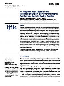
Fig. 1 the UAV is provided with five control surfaces and throttle. In the presence of an actuator failure these various controls provide redundancies which allow to keep the aircraft in flight. d r > 0

E le v a to r d r o it

d e r

A ile r o n d r o it

R u d d e r

d a r

d a l > 0

The UAV Mistral and its 6 actuators

A nonlinear model of the UAV supposed rigid body and constant weight is built around a six degrees of freedom platform. The state vector X = [ϕ, θ, V, α, β, p, q, r, Z]T where ϕ is the bank angle, θ the trim, V the true airspeed, α the angle of attack, β the sideslip, p, q, r roll, pitch and yaw, Z the height. The control vector U = [δx , δar , δal , δer , δel , δr ]T where δx is the throttle, δar , δal the right and left ailerons, δer et δel the right and left elevators and the rudder δr . For this aircraft, all the state vector is measured. The UAV equations issued from aircraft flight mechanics are nodetailed in this paper, but they can be represented by the following nonlinear equations : X˙ Y

= f (X) + g(X)U = X

(1)

When the UAV flies level, (1) is linearized around a operating point {Xe , Ue }, the model of the aircraft becomes : x˙ = Ax + Bu y

(2)

= x

The state matrix A : 

Aϕϕ  Aθϕ  Avϕ  Aαϕ  Aβϕ  0   0  0 Azϕ

Aϕθ 0 Avθ Aαθ Aβθ 0 0 0 Azθ

0 0 Avv Aαv Aβv Apv Aqv Arv Azv

0 0 Avα Aαα 0 Apα Aqα Arα Azα

0 0 Avβ Aαβ Aββ Apβ 0 Arβ Azβ

Aϕp 0 0 Aαp Aβp App Aqp Arp 0

Aϕq Aθq 0 Aαq 0 Apq Aqq Arq 0

Aϕr Aθr 0 Aαr Aβr Apr Aqr Arr 0

 Bθδx  Bvδ  x Bαδx B  βδx  0   0  0

0 0

0 0

0 0

0 0

Bvδar Bαδar 0 Bpδar Bqδar Brδar 0

Bvδal Bαδal 0 Bpδal Bqδal Brδal 0

Bvδer Bαδer 0 Bpδer Bqδer Brδer 0

Bvδel Bαδel 0 Bpδel Bqδel Brδel 0

0



Bθδr  0   Bαδr   Bβδr  Bpδr   Bqδr   Brδr 0

In this UAV, two controllers (Fig. 2) are set up for the longitudinal and for the lateral-directional state variables. They are carried out using eigenstructure assignment technique. As far as the longitudinal axis is concerned, the UAV disposes of two control inputs : elevators and throttle, thus an external closed-loop control with proportional-integral controller is designed for true airspeed and height. As regards the lateral axis, the only output controlled is the bank angle.

d x

Fig. 1.

0

0

d e l > 0

P r o p u ls io n

The control matrix B : 



0 0 0  0  0 0  0  0 0

ϕc + −

6

R

[δar , δal , δr ] - Llat -+ - lateral model − 6 Klat ¾

[Vc , Zc ]T R + − 6

[δx , δer , δel ] -Llon -+ - longi model − 6

- Clat ϕ

− [φ, β, p, r] T

-Clon [V, Z]

KLon ¾ [V, α, β, q, Z]

Fig. 2.

The lateral and longitudinal closed-loops

III. UNKNOWN INPUT DECOUPLED FUNCTION OBSERVER In this part, results established in [1] are recalled. The following dynamic system driven by both known and unknown input is considered : ½ x˙ = Ax + Bu + Gd (3) y = Cx where x ∈ Rn is the state, u ∈ Rm is the known input, d ∈ Rq is the unknown input and y ∈ Rp the output. A, B, G and C are matrices with appropriate dimensions. Moreover G and C are assumed to be full rank. The Unknown Input Decoupled Functional Observer (UIDFO) proposed in [1] is described by the following equations : ½ z˙ = F z + Ly + T Bu + T Gdˆ (4) dˆ = γ(W y − N z) γ ∈ R∗+

where γ is a positive scalar, z is an estimate of linear combination of state T x and dˆ is the estimate of d. Matrices F, T, L, N and W are all design parameters that need to be set in order to satisfy the following conditions : F T − T A + LC = 0

F is stable

N = (T G)T P P F + F T P = −Q (5)

P verifies : T

T

easily set as identity matrix. Indeed, according to the algorithm, Kd is choosen in order to get Aˆd stable. Moreover, if Kd is choosen in order to get Aˆd diagonal, then Fd = diag(λ(Aˆd )) = Aˆd , hence Vd = Iq . Next a tuning of the matrices Fd and Pd is proposed such that, H(0) → Iq and bandwidths of each of the ˆ i (s) D transfer functions hii (s) = D are controlled. Paramei (s) ter γ is useless and is set equal to one. the static gain is given by : −1 −T −1 −1 Γ3 H(0) = Γ−T 3 Pd (−Fd + Γ3 Γ3 Pd )

(6)

NT = G T PT = WC rank(T G) = rank(G) = q These matrices exist if and only if, (i) rank(CG) = rank(G), (ii) All unstable transmission zeros of system (A, G, C) are unobservable modes of (A, C). To proof the existence and to compute these matrices, system (A, G, C) is transformed into Special Coordinate Basis (SCB) [13], [14]. The design algorithm of the observer proposed in [1] useful to understand the following sections is in appendix VII-A. However the authors of [1] mentioned that the setup of the observer remains an open problem. In this paper, a modification of this algorithm is proposed in order to set the dynamic observer. A. Tuning of the UIDFO The role of this observer is to estimate the unknown input d and its is proved in [1] that : ˆ D(s) = H(s)D(s) with H(s) ∈ Rq×q the transfer function between D(s) ˆ the Laplace transform of d(t) and D(s) the Laplace ˆ transform of d(t) the estimate of d(t) where : −1 −T T T −1 H(s) = γΓ−T Vd Γ−1 3 Vd Pd (sI−Fd +γVd Γ3 Γ3 Vd Pd ) 3

The estimation of unknown input dˆ converges on unknown input d if the modulus of the transfer function kH(jω)k tends towards identity matrix Iq . According to [1], this can be reached if γ → +∞. However, the bandwidth of the observer increase with γ, consequences of this is the rise of noise sensibility. In this paper a tuning of the observer such as kH(jω)k = Iq in a given bandwidth and kH(jω)k → 0 outside is proposed. As the algorithm shows, there are few constraints to choose matrices Fd and Qd . Eigenvalues of Fd are set negative and Qd is positive-definite. Still, these two matrices determine static gains and bandwidths of the transfer functions of H(s) (indeed, given Qd , Pd is the Lyapunov matrix of Fd ). Γ3 and Vd are not used to set the observer parameters. Γ3 is G transformation in SCB, as for Vd , it can be

the transfer functions bandwidths hii (s) of the observer are characterized by the eigenvalues of : −T (Fd − Γ−1 3 Γ3 P d )

(7)

with the matrix inversion lemma, (6) is rewritten : −1 −1 −1 H(0) = Iq + (Γ−T 3 P d F d Γ 3 − Iq )

(8)

This result is proved in appendix VII-B. The problem consists in determining the q cœfficients of the diagonal matrix Fd and the q × q cœfficients of the matrix Pd which minimize the square modulus of each one of the terms ∆hij (0) of : −1 −1 −1 ∆H(0) = (Γ−T 3 Pd Fd Γ3 − Iq )

(9)

whereas the eigenvalues of (7) are placed according to the desired observer dynamic under the constraints : Fd Pd Pd FdT + Fd Pd

negative definite symmetric positive definite (SPD) SPD

This problem is solved whith the constrainted optimization MATLAB function fmincon. The cost function to minimize is :

J=

q,q X

|∆hij (0)|2 +

i,j=1

q µ X

k=1

¶2 −T P ) Γ λdk −λk (Fd −Γ−1 d 3 3 (10)

where λdk is the k ith desired eigenvalue. Constraints are expressed as follows : M ∈ Rq is SPD if and only if the following matrices (the leading principal minors) have positive determinant, |M1 | |M2 | ... |Mq |

> 0 > 0 ... > 0

Here this result is applied to matrices −Fd , Pd and Pd FdT + Fd Pd .

IV. FAULT DIAGNOSIS SYSTEM PERFORMED WITH AN UIDFO The UIDFO described above is used here to solve the problem of actuator fault diagnosis. In the following, u is the really input vector applied to the UAV, u ¯ is the input vector calculated by the controllers and u ˆ the input vector estimated by the UIDFO. The UIDFO estimates UAV actuator positions u ˆ of u and a comparison with controlled inputs u ¯ provided by the two controllers is made. Note that these latest (¯ u) are processed to take into account saturations of the actuators. In fault free mode, the actuators carry out the controlled inputs and u = u ¯. When an actuator failure occurs u ˆ 6= u ¯, the difference u ˆ−u ¯ is compared with a threshold σu which is interpreted by a detection and isolation logic. Because of the actuator redundancies, matrix B (which plays role of G)is not full rank and a unique observer is not sufficient to estimate all the inputs. Hence two observers are required to estimate the six actuator positions as shows Fig. 3.

where B1 plays role of B and B2 plays role of G. When one of the inputs δ1i in u1 (resp δ2i in u2 ) breaks down, observer 1 (resp observer 2) gives an estimation u ˆ1 (resp u ˆ2 ) of the healthy and faulty inputs of vector u1 (resp u2 ). The faulty input δ1i (resp δ2i ) can be easily isolated because its estimate δˆ1i (resp δˆ2i ) is the only one which is different from the input δ¯1i (resp δ¯2i ) calculated by the contollers. Let µδ1i a logic state linked with the difference |δˆ1i − δ¯1i | and σδ1i a threshold such that :

|δˆ1i − δ¯1i | > σδ1i =⇒ µδ1i = 1 |δˆ1i − δ¯1i | ≤ σδ1i =⇒ µδ1i = 0

(13)

Let δif the ith faulty input. The following incidence matrix may be implemented to isolate the failure, TABLE I The incidence matrix

Observer 2 -

y u ¯1

-

|εu2 | u2 u ˆ2 + ε|.| -+ -6

Detection

σu2

Isolation

σu1 u ¯2

-

--? ε - u1- |.| -+ u ˆ1+ |εu1 |

-

ufi -

Logic

Observer 1 Fig. 3.

Fault Detection Isolation system built whith 2 UIDFO

Matrix B is rewritten B = [B1 , B2 ]. The first UIDFO named observer 1 estimates the input vector u ˆ1 which is an estimation of the actuator positions u1 = [δx , δar , δer ]T . It uses the output y and the input vector u ¯2 = [δ¯al , δ¯el , δ¯r ]T calculated by the controllers. The equations of the first observers issued from (4) is : ½ z˙1 = F1 z1 + L1 y + T1 B2 u ¯2 + T1 B1 u ˆ1 (11) u ˆ1 = (W1 y − N1 z1 ) where B2 plays role of B and B1 plays role of G. The second named observer 2 estimates the second input vector u ˆ2 which is an estimation of the actuator positions u2 = [δal , δel , δr ]T . It uses the output y and the input u ¯1 calculated by the controllers. The equations of the second observer issued from (4) is : ½ z˙2 = F2 z2 + L2 y + T2 B1 u ¯1 + T2 B2 u ˆ2 (12) u ˆ2 = (W2 y − N2 z2 )

δxf f δar f δer f δal f δel δrf

µ δx 1 0 0 1 1 1

µδar 0 1 0 1 1 1

µδer 0 0 1 1 1 1

µδal 1 1 1 1 0 0

µδel 1 1 1 0 1 0

µ δr × × × 0 0 1

Suppose a failure occurs on u1 (resp u2 ). To provide an estimation, observer 2 (resp observer 1) uses the controlled input vector u ¯1 (resp u ¯2 ). As this vector is different from the really applied input vector u1 (resp u2 ), its estimate u ˆ2 (resp u ˆ1 ) is wrong. So, when the actuator failure has been detected and isolated, its estimate δˆ1i (resp δˆ2i ) may be used instead of δ¯1i (resp δ¯2i ). Thus the observer 2 (resp observer 1) exploits a faithful information and provides a correct estimation of the unknown inputs.

V. SIMULATIONS Fig. 4 shows the Bode magnitude diagram of the observer 1 dedicated to estimate inputs δx , δar and δer . The three desired eigenvalues of matrix (7) are −1000. Modulus of these eigenvalues, obtained with the tuning method presented above are 1037, 1037 and 1045 and, as expected H(0) tends towards I3 , 

0.9670 H(0) = 0.0030 0.0073

0.0054 0.9944 0.0112

 0.0144 0.0024 0.9885

Bode Diagram

From: δ

From: δ

x

From: δ

ar

When a control surface sticks, the estimation of the faulty input is used to compute a new operating point. Next a new controller may be implemented in order to maintain in flight the aircraft. First simulations performed with assymetric elevator failure are promising.

el

To: δ est x

0 -20 -40

To: δ est ar

Magnitude (dB)

-60 0

-50

δx

δal

0.5

-100 0

0.4

1

real inputs estimated inputs

0.5

To: δ est el

0.3

0

0.2

-20

-0.5

0.1

-40

0 0

-60

0

5

10

10

0

5

10

0

10

-1 5

10

15

20

10

30

35

40

45

50

28

30

32

34

36

δar

5

10

25

38

40

42

44

46

48

50

δel

1

10

Frequency (rad/sec)

Fig. 4.

Bode magnitude diagrams of the observer

0

0

-1

-10

-2 0

5

10

15

20

25

30

35

40

45

50

-20 0

5

10

15

20

δer

The FDI presented above has been implemented on the nonlinear model of the UAV. Simulation results on Fig. 5 show the six real inputs u and their estimated u ˆ. The UAV flies level in normal mode for the time interval [0, 40s], the true airspeed reference is modified and the elevator position is varying between −5◦ and −6◦ . At t = 40s, the right elevator breaks down and δer = 0◦ . As δer is in u1 , the observer 1 gives a correct estimation u ˆ1 of u1 . On the other hand, δ¯er in u ¯1 is calculated with the longitudinal regulator and is different from δer in u1 which is locked. As observer 2 uses u ¯1 , Fig. 5 shows that estimations δˆel and δˆal in u ˆ2 are wrong. δx

δal

0.5 0.4

1

real inputs estimated inputs

5

2

0

1

-5

0

-10 0

-1 0

0.2

10

15

20

25

30

Fig. 6.

30

35

40

45

50

35

40

45

50

5

10

15

20

25

30

35

40

45

50

Input estimations with correction

References [1]

Y. Xiong and M. Saif, Unknown disturbance inputs estimation based on state functional observer design, Automatica 39, pp. 1390-1398, 2003.

[2]

Office of the Secretary of Defense, Unmanned Aerial Vehicle Reliability Study, february 2003.

[3]

C. Hajiyev, F. Caliskan, Sensor and control surface/actuator failure detection applied to F16 flight dynamic, Aircraft Engineering and aerospace technology (2), 2005, pp.152-160.

[4]

M. Napolitano, Y. Song, B. Seanor, On-line parameter estimation for restructurable flight control system, Aircraft Design (4), 2001, pp.19-50.

[5]

S. Glavaˇski, G. Papageorgiou, M.Elgersma, P. Lommel, Active failure management for aircraft control recovery, AIAA Guidance, Navigation and Control Conference and Exhibit, August 2002.

[6]

A. Marcos, S. Ganguli, G.J. Balas, An application of H∞ fault detection and isolation to a transport aircraft, Control Engineering Practice (13), 2005, pp.105-119.

[7]

M. Napolitano, Y. An, B. Seanor, A fault tolerant flight control system for sensor and actuatot failures using neural network, Aircraft Design (3), 2000, pp.103-128.

[8]

J.L. Aravena, F.N. Chowdhury, Fault detection of flight critical systems in Proc. 20th , Digital Avionics Systems Conference, October 2001.

[9]

T. Kobayashi and D.L. Simon, Application of a bank of Kalman filters for aircraft engine fault diagnostics, NASA Report 212526, 2003.

0

0.3

5

25

δr

-1

0.1 0 0

10

20

30

40

50

60

-2 0

10

20

δar

30

40

50

60

δel 10

0 0 -0.5 -10 -1 30

35

40

45

50

55

60

-20 0

10

20

δer 5

2

0

1

-5

-10 0

30

40

50

60

δr

0

10

20

30

40

Fig. 5.

50

60

-1 0

10

20

30

40

50

60

Real and estimated inputs

The case presented on Fig. 6 is the same as above. However, when a fault occurs, it is detected by the decision logic which commutates δˆer instead of δ¯er on the observer 2. As this observer uses a faithful information, a correct estimation u ˆ2 of u2 is given. VI. CONCLUSIONS AND FUTURE WORKS In this paper, input observers able to estimate actuator positions of an UAV were carried out. They were associated with a fault detection and isolation logic. Moreover, a tuning method of the dynamic observer has been proposed. Current work is focused on FDI implementation with a fault tolerant control system.

[10] G. Ducard, A Reconfigurable Flight Control System based on the EMMAE Method, ACC Conf. 2006, pp.5499-5504. [11] M.Hou and R.J. Patton, Input observability and input reconstruction, Automatica 34, pp.789-794, 1998. [12] M. Corless and J. Tu, State and input estimation for a class of uncertain systems, Automatica 34, pp.757-764, 1998. [13] B.M. Chen, On properties of the special coordinate basis of linear system, International Journal of Control, 71, 1998, pp.981-1003. [14] X.Liu, B.M. Chen and Z. Lin, Linear system toolkit in MATLAB : structural decomposition and their applications, Journal of Control, theory and application, 3, 2005, pp. 287-294.

VII. appendix A. Algorithm 1) Conditions (i) and (ii) being satisfied, A, G, C d´efined in (1) are expressed in the Special Coordinates ¯ Basis 1 . The structures of the matrices C¯ and G take into account the fact that nc = 0 and that all infinite-zero degrees are one.  −  − Aaa 0 L− ab Cb Lad + +   0 A+ aa Lab Cb Lad  A¯ = Γ−1 =  1 AΓ1  0 0 Abb Lbd  − Eda 0 Edb Ad ¯ = G

Γ−1 1 GΓ3

  0 0  =  0 Iq

C¯

Γ−1 2 CΓ1

=

=

µ

0 0 0 0

0 Cb

Iq 0

¶

2) Compute Kb and Kd such that Aˆb = Abb − Kb Cb and Aˆd = Ad − Kd are stable matrices. Then ¯ such that, compute K  −  Lad L− ab +  + ¯ = Lad Lab  K  Lbd Kb  Kd 0 λ(Aˆb ) and λ(Aˆd ) 3) Calculate the eigenvalues ¯ C¯ and which are among the eigenvalues of A¯ − K their associated left-eigenvectors : λ(A− aa ),

[Va− , 0, 0, 0], [0, 0, Vb , 0], [Vad , 0, Vbd , Vd ] Then construct   λ(A− 0 0 aa ) λ(Aˆb ) 0  F¯ =  0 0 0 λ(Aˆd )  −  Va 0 0 0 ¯ = T¯K ¯ 0 , L T¯ =  0 0 Vb Vad 0 Vbd Vd Let Vab =

Fab

µ

Va− 0

0 Vb

¶

¡ Vdd = Vad

Vbd

¢

µ ¶ ¡ ¢ λ(A− 0 aa ) = Fd = λ(Aˆd ) 0 λ(Aˆb )

4) Given any SPD matrix Qd , calculate P d which is solution of the Lyapunov equation : Pd Fd + FdT Pd = −Qd . At this point, the modifications suggested above (III-A) may be used to compute these matrices. 1 A toolbox proposed by [14] may be downloaded at http ://linearsystemskit.net

−1 5) Calculate Pbd = −Pd Vdd Vab and Qbd = T −(Pbd Fab + Fd Pbd ). 6) Choose α ∈ R∗+ which is large enough and calculate Pab by solving : T −αI = Pab Fab + Fab Pab

check that, |λmax (α−1 Qbd QTbd Q−1 d )| < 1 −1 T −1 Pbd Pd )| < 1 |λmax (Pbd Pab

Finally, assemble P as : µ ¶ T Pab Pbd P = Pbd Pd ¯ = (T¯G) ¯ T P and W ¯ = (T¯G) ¯ T P T¯C¯ † 7) Calculate N † ¯ ¯ where C is the pseudo-inverse of C. 8) Calculate F, T, L, N for original system matrices as F = F¯ T = T¯Γ−1 1 ¯ N = Γ−T N 3

¯ −1 W = Γ−T 3 W Γ2 ¯ −1 L = LΓ 2 B. Calculus of H(0) We establish with the matrix inversion lemma that : −1 −T −1 −1 H(0) = Γ−T Γ3 3 Pd (−Fd + Γ3 Γ3 Pd )

equals : −1 −1 −1 H(0) = Iq + (Γ−T 3 P d F d Γ 3 − Iq )

The matrix inversion lemma : −1 = (A11 − A12 A−1 22 A21 ) −1 −1 −1 A−1 A21 A−1 11 + A11 A12 (A22 A11 A12 ) 11

H(0) has the form : H(0) = C(BC − Fd )−1 B with B = Γ−1 et C = Γ−T 3 3 Pd . To get a formulation similar as the matrix inversion lemma form, H(0) is written : H(0) = C(BC − Iq Iq Fd )−1 B According to the lemma : H(0) = ¢ ¡ C (BC)−1 + (BC)−1 Iq (Iq−1 − Fd (BC)−1 Iq )−1 Fd (BC)−1 B ¡ ¢ = C (BC)−1 + (BC)−1 (Iq − Fd (BC)−1 )−1 Fd (BC)−1 B ¡ ¢ = C C −1 B −1 + C −1 B −1 (Iq − Fd (BC)−1 )−1 Fd C −1 B −1 B = Iq + B −1 (Iq − Fd (BC)−1 )−1 Fd C −1 ¡ ¢−1 = Iq + (Fd C −1 )−1 (Iq − Fd (BC)−1 )B ¡ ¢−1 = Iq + CFd−1 (Iq − Fd C −1 B −1 )B ¡ ¢−1 = Iq + CFd−1 B − CFd Fd−1 C −1 B −1 B ¢−1 ¡ = Iq + CFd−1 B − Iq ¡ ¢−1 −1 −1 = Iq + Γ−T 2 3 Pd Fd Γ3 − Iq

C. Matrices A and B Aϕp

=

1

Aϕq

=

sin ϕe tan θe

Aϕr

=

cos ϕe tan θe

Aϕϕ

=

qe cos ϕe − re sin ϕe tan θe

Aϕθ

=

Aθq Aθr

=

qe sin ϕe + re cos ϕe 2 cos θe cos ϕe

=

− sin ϕe

Aθϕ Azv

=

−qe sin ϕe − re cos ϕe

=

− sin θe cos αe cos βe + sin ϕe cos θe sin βe + sin αe cos βe cos ϕe cos θe

Azβ

=

Ve (sin θe cos αe sin βe + sin ϕe cos θe cos βe − sin αe cos ϕe cos θe sin βe )

Azα

=

Ve (sin θe cos βe sin αe + cos βe cos ϕe cos θe cos αe )

Azϕ

=

Ve (cos θe sin βe cos ϕe − sin αe cos βe cos θe sin ϕe )

Azθ

=

−Ve (cos θe cos αe cos βe + sin ϕe sin βe sin θe + sin αe cos βe cos ϕe sin θe )

Avv

=

−2

qS ¯ ref mVe

(Cxe +

X i

Cxδ δi ) − i e

F xprop0 cos(αe ) cos(βe )δxe (mVe )

Avβ

=

g(cos αe sin θe sin βe + cos θe sin ϕe cos βe − sin αe sin βe cos θe cos ϕe ) −

Avα

=

g(cos βe sin θe sin αe + cos αe cos βe cos θe cos ϕe ) −

Avϕ

=

g(sin βe cos θe cos ϕe − sin αe cos βe cos θe sin ϕe ) −g(cos αe cos βe cos θe + sin αe cos βe sin θe cos ϕe + sin βe sin ϕe sin θe )

m F xprop0 sin αe cos βe δxe

qS ¯ ref Cxα m

F xprop0 cos αe sin βe δxe

−

m

Avθ

=

Aβv

=

Aββ

=

Aβp Aβr

=

(sin βe cos θe sin ϕe − cos αe cos βe sin θe + sin αe cos βe cos θe cos ϕe ) + Ve sin αe

=

− cos αe

Aβϕ

=

Aβθ

=

−g Ve2 −g

g Ve −g Ve

Aαv

=

Aαβ

=

Aαα

=

(cos βe cos θe sin ϕe + cos αe sin βe sin θe − sin αe sin βe cos θe cos ϕe ) +

qS ¯ ref Cy βe mVe2 qS ¯ ref Cyβ mVe

+

e −

2F xprop0 cos αe sin βe δxe mVe2 F xprop0 cos αe cos βe δxe

(cos βe cos θe cos ϕe + sin αe sin βe cos θe sin ϕe ) (cos βe sin θe sin ϕe − cos αe sin βe cos θe − sin αe sin βe sin θe cos ϕe )

qS ¯ ref X 2F xprop0 sin αe δxe Czδ δi ) + (Cze + i e mVe2 cos βe mVe cos βe i (pe cos αe + re sin αe ) (sin αe sin θe + cos αe cos θe cos ϕe ) − 2 2 Ve cos βe cos βe qS ¯ ref sin βe X F xprop0 sin αe sin βe − Czδ δi ) − (Cze + i 2 2 mVe cos βe mVe cos βe i qS ¯ ref Czα F xprop0 cos αe δxe g (cos αe sin θe − sin αe cos θe cos ϕe ) + (pe sin αe − re cos αe ) tan βe − − Ve cos βe mVe cos βe mVe cos βe − cos θe tan βe −g

Ve2 cos βe g sin βe

(sin αe sin θe + cos αe cos θe cos ϕe ) −

=

Aαq

=

1

Aαr

=

Aαθ

=

Aαϕ

=

Apv

=

Apβ

=

Apα

=

App

=

− sin αe tan βe g sin αe cos θe − cos αe sin θe cos ϕe Ve cos βe −g cos αe cos θe sin ϕe Ve cos βe bref re ´ bref pe qS ¯ ref bref ³ X + Clr Clδ δi ) + Clp 2J11 (Clβ + e 2V e e i e Ve 2Ve e i ³ bref re ´ bref pe X + Cnre + 2J13 (Cnβ βe + Cnδ δi ) + Cnpe e e ie 2Ve 2Ve i ³ qS ¯ ref bref J11 Clβ + J13 Cnβ ) e e ³ bref re bref pe bref re ´ bref pe + Clr ) + J13 (Cnβα βe + Cnpα + Cnrα ) qS ¯ ref bref J11 (Clβ βe + Clp α α e 2Ve Ve 2Ve 2Ve ³ ´ bref bref qS ¯ ref bref J11 Clp + J13 Cnpe + (J11 Izx + J13 (Ixx − Iyy))qe e 2V 2Ve e ´ ³ J11 (Iyy − Izz)re + Izxpe ) + J13 ((Ixx − Iyy)pe − Izxre

Apq

= =

Aqv

=

Aqα

=

Aqp

=

Aqq

=

Aqr

=

Arv

=

Arβ Arα

´ ³ bref bref + J13 Cnre + (J11 (Iyy − Izz) − J13 Izx)qe qS ¯ ref bref J11 Clr e 2V 2Ve e qS ¯ ref cr ef ³ cref qe ´ X J22 δi δi ) + Cm 2(Cme + e Ve 2Ve i J22 qS ¯ ref cref Cmαe ´ ³ J22 (Izz − Ixx)re − 2Izxpe cref J22 qS ¯ ref cref Cmq 2Ve ´ ³ J22 (Izz − Ixx)pe + 2Izxre qS ¯ ref bref ³ Ve

= =

Arp

=

Arq

=

Arr

=

qS ¯ ref Cyδ δre r mVe2

mVe

Aαp

Apr

+

2J31 (Clβ βe + e

qS ¯ ref bref (J31 Clβ

e

X i

Clδ δi ) + J31 (Clp e i e

bref pe 2Ve

+ Clr e

bref re 2Ve

) + 2J33 (Cnβ βe + e

X i

Cnδ δi ) + J33 (Cnpe i e

+ J33 Cnβ ) e

bref re bref pe bref re ´ + Clrα ) + J33 (Cnβα βe + Cnpα + Cnrα ) 2Ve 2Ve 2Ve Ve ³ ´ bref bref qS ¯ ref bref J31 Clp + J33 Cnpe ) + (J31 Izx + J33 (Ixx − Iyy))qe ) e 2V 2Ve e J31 ((Iyy − Izz)re + Izxpe ) + J33 ((Ixx − Iyy)pe − Izxre ) ³

qS ¯ ref bref J31 (Clβα βe + Clpα αe

bref pe

´ ³ bref bref + J33 Cnre ) + J31 (Iyy − Izz) − J33 Izx)qe qS ¯ ref bref (J31 Clr e 2V 2Ve e

bref pe 2Ve

+ Clr e

bref re ´ ) 2Ve

Bvδ

x

Bvδ Bβδ

i

x

Bβδ Bαδ

r

x

Bαδ

i

Bpδ i Bpδ r Bqδ i Brδ i Brδ r

=

F xprop0 cos αe cos βe m qS ¯ ref Cx δi

=

−

=

−

= =

m F xprop0 cos αe sin βe

mVe qS ¯ ref Cyδr mVe F xprop0 sin αe

−

=

mVe cos βe qS ¯ ref Cz δi mVe cos βe qS ¯ ref bref (J11 Clδ

=

qS ¯ ref bref J13 Cnδ

=

−

i

+ J13 Cnδ ) i

r

=

qc ¯ ref Sref J22 Cmδ

=

qb ¯ ref Sref (J31 Clδ

=

qb ¯ ref Sref J33 Cnδ

i

i

r

+ J33 Cnδ ) i