IEEE TRANSACTIONS ON MEDICAL IMAGING, VOL. 22, NO. 9, SEPTEMBER 2003
1063
An Adaptive Spatial Fuzzy Clustering Algorithm for 3-D MR Image Segmentation Alan Wee-Chung Liew*, Member, IEEE, and Hong Yan, Senior Member, IEEE
Abstract—An adaptive spatial fuzzy c-means clustering algorithm is presented in this paper for the segmentation of three-dimensional (3-D) magnetic resonance (MR) images. The input images may be corrupted by noise and intensity nonuniformity (INU) artifact. The proposed algorithm takes into account the spatial continuity constraints by using a dissimilarity index that allows spatial interactions between image voxels. The local spatial continuity constraint reduces the noise effect and the classification ambiguity. The INU artifact is formulated as a multiplicative bias field affecting the true MR imaging signal. By modeling the log bias field as a stack of smoothing -spline surfaces, with continuity enforced across slices, the computation of the 3-D bias field reduces to that of finding the -spline coefficients, which can be obtained using a computationally efficient two-stage algorithm. The efficacy of the proposed algorithm is demonstrated by extensive segmentation experiments using both simulated and real MR images and by comparison with other published algorithms. Index Terms—Adaptive spatial fuzzy clustering, intensity nonuniformity correction, MR image segmentation, spatial continuity constraint, spline approximation.
I. INTRODUCTION
A
N IMPORTANT first step in image analysis is image segmentation, or separation of the input image into meaningful regions. In medical imaging, this could involve organ detection or tissue characterization. A commonly used image segmentation method is the fuzzy c-means (FCM) clustering algorithm [1]–[4], which assigns pixels in the image into different classes according to their features. In image segmentation, we expect the pixels in the same class to have similar pixel values independent of their locations. However, in magnetic resonance imaging (MRI), inhomogeneity in the magnetic field usually give rises to the so-called intensity nonuniformity (INU) artifact [5]. This common artifact exhibits itself as a smooth, slowly varying change in image pixel values and could have adverse effect on the performance of intensitybased automatic segmentation methods [37], [38]. In addition to intensity variation due to field inhomogeneity, there may be
Manuscript received June 29, 2001; revised March 18, 2003. This work was supported by the Hong Kong Research Grant Council under Project CityU 1088/00E. The Associate Editor responsible for coordinating the review of this paper and recommending its publication was C. Meyer. Asterisk indicates corresponding author. *A. W. C. Liew is with the Department of Computer Engineering and Information Technology, City University of Hong Kong, Hong Kong (e-mail:
[email protected]). H. Yan is with the Department of Computer Engineering and Information Technology, City University of Hong Kong, Hong Kong, and School of Electrical and Information Engineering, University of Sydney, NSW 2006, Australia (e-mail:
[email protected]). Digital Object Identifier 10.1109/TMI.2003.816956
a lack of tissue specific meanings for MRI intensities within scans, even for the same patient obtained on the same scanner using the same protocol. Data preprocessing using a tissue intensity calibration procedure as proposed in [6] prior to the segmentation process would ensure a more accurate segmentation. Besides INU artifact, issues such as poor contrast and imaging noise also make accurate segmentation difficult. In addition, many pixels in a real image are ambiguous and cannot be classified consistently based on feature attributes alone. In an image, pixels of the same object usually form coherent patches. Thus, the incorporation of local spatial information in the clustering process could filter out noise and artifacts and reduce classification ambiguities. Several methods have been proposed to correct the INU artifact [7]–[15], [30]–[33]. In [7], [8], and [11], a polynomial surface and a thin-plate spline surface are used to approximate the bias field associated with the INU, respectively. In [9], the bias field for the INU is estimated by sharpening the image histogram in an iterative process. In these methods, after correcting the INU artifact, the MR image is then segmented using an algorithm that assumes that the inhomegeneity is not present. In [12], [13], and [33], the bias field is estimated by homomorphic filtering. In [10], the problem of estimating the bias field is cast in a Bayesian framework and the EM algorithm is used to estimate the inhomogeneity and the tissue classes. In [39] and [40], the MRI brain tissue classes are modeled as finite Gaussian mixtures with Markov random field regularization for contextual information and a priori digital brain atlas initialization, whereas the bias field is modeled as a fourth order least square polynomial fit. A method of estimating the INU based on fuzzy clustering has been reported in [15], where intermediate segmentation results are utilized for the INU estimation. The method uses a modified FCM cost functional to model the variation in intensity values via a multiplicative bias field applied to the cluster centroids. The computation of the bias field is formulated as a variational problem and the bias field is estimated at every voxel using a multigrid algorithm. Many attempts have also been made to introduce spatial context into the classification and segmentation procedures. One popular approach is the relaxation labeling method [16]–[18]. However, relaxation labeling requires the initial labeling probabilities of each pixel to be available. In [19], a spatial continuity constraint is incorporated into the fuzzy clustering algorithm by either the addition of a small positive constant to, or subtraction of a small positive constant from, the membership value of the center pixel in a 3 3 window. The decision depends on whether the optimal cluster assignment for the pixel in the 8-neighborhood is the same as, or different from, that
0278-0062/03$17.00 © 2003 IEEE
1064
IEEE TRANSACTIONS ON MEDICAL IMAGING, VOL. 22, NO. 9, SEPTEMBER 2003
of the center pixel. Recently, a supervised segmentation technique using the idea of fuzzy-connectedness has been proposed in [21] and [22], which take into account pixel affinities and spatial continuities using the notion of fuzzy “hanging togetherness.” Given some prelabeled pixels from each of the object classes, the fuzzy-connectedness map of pairs of pixels is computed. The segmentation can then be obtained by appropriate thresholding of the fuzzy-connectedness map. In this paper, we proposed an FCM-based algorithm that addresses both the INU artifact and the local spatial continuity. Our method incorporates the local spatial continuity into the clustering algorithm using a dissimilarity index [20], in place of the usual distance metric. The log of the three-dimensional (3-D) multiplicative bias field is modeled by a stack of smoothing -spline surfaces and estimated by an efficient two-stage algorithm. Although the method in [15] is also FCM-based, our approach is different in several aspects. First, the bias field is derived according to the commonly used multiplicative model [7]–[11], [14]. Second, the 3-D log bias field is modeled as a stack of smoothing -spline surfaces, instead of the solution to a variational problem. Finally, the spatial continuity constraint is taken into account in our fuzzy objective function. Extensive experiments using both simulated and real MR brain image data show that the proposed algorithm can suppress INU and noise to produce good segmentation results. II. PROBLEM FORMULATION The task of 3-D MR image segmentation involves the separation of image voxels into regions comprising different tissue be the 3-D image coordinate of a voxel. types. Let We assume that each tissue class has a specific value , that would is, a quantity being measured. Then, the ideal signal consist of piecewise constant regions,1 each having one of the values. However, imperfection in the magnetic field often introduces an unwanted low frequency bias term into the signal, which gives rise to the INU artifact. The bias field that gives rise to the INU artifact in an MR image is usually modeled as a smooth multiplicative field. This model is widely used [7]–[11], [14] and is consistent with the spatial inhomogeneity arising from the variation in the sensitivity of the RF coils and the nonuniform excitations. The image formation process in MRI can be modeled as (1) is the measured MR signal, is the true signal where is the unknown smoothly varying bias emitted by the tissue, is an additive noise assumed to be independent field, and . Accurate segmentation of an MR image thus involves of and rean accurate estimation of the unknown bias field moving this bias field from the measured MR signal. Using the
estimated as
, the log-transformed true signal can be recovered
(2)
III. METHODS A. Conventional FCM Segmentation The FCM clustering algorithm assigns a fuzzy membership value to each data point based on its proximity to the cluster be the set centroids in the feature space [1]. Let of feature vectors associated with a 3-D image defined in the domain . The conventional FCM algorithm is formulated as with respect the minimization of the objective functional to the membership values and cluster centroids
(3) is a fuzzy c-partition of , is the set of fuzzy cluster centroids, is the fuzzy index, is the total number of clusters, gives the membership of pixel in the th cluster and . Using the Euclidean norm, the distance metric measures the vector distance of a feature vector from a cluster centroid in the feature space, i.e.,
where the matrix
(4) The FCM objective function is minimized when high memthat are close to the cenbership values are assigned to troid for their particular class, and low membership values are assigned when they are far from the centroid. Letting the first with respect to and equal to zero yields derivatives of . The FCM the two necessary conditions for minimizing algorithm proceeds by iterating the two necessary conditions until a solution is reached. After FCM clustering, each data sample will be associated with a membership value for each class. By assigning the data sample to the class with the highest membership value, a segmentation of the data can be obtained. In the conventional FCM formulation, each class is assumed to have a uniform value as given by its centroid. Each data point is also assumed to be independent of every other data point and spatial interaction between data points is not considered. However, for image data, there is strong correlation between neighboring pixels. In addition, due to the INU artifact, the data in a class no longer have a uniform value. Therefore, to produce meaningful segmentation, the conventional FCM algorithm has to be modified to take into account both local spatial continuity between neighboring data and INU artifact compensation. B. Incorporation of Local Spatial Continuity
1In
practice, the limited resolution of the imaging device leads to blurring along border regions between tissue classes, i.e., the partial volume effect. However, this effect is confined to the border regions, in contrast to the more global INU artifact.
The incorporation of local spatial continuity considers the influence of neighboring voxels on the center voxel of interest denote a chosen 3-D local during classification [20]. Let
LIEW AND YAN: ADAPTIVE SPATIAL FUZZY CLUSTERING ALGORITHM FOR 3-D MR IMAGE SEGMENTATION
neighborhood configuration with respect to a center voxel . and the center voxel belong to the same If the voxels in class, then should be smoothed by the clustering results of its neighboring voxels so that they all eventually have high and similar membership values in one of the clusters. This is done denote the distance as follows. Let in the 3-D MR between vectors and . For every voxel distances image, we compute the following (5) (6) is the neighborhood of and is the centroid of where is small, we would like the th cluster. Now, if the distance to be greatly influenced by . Otherwise, should . Taking all voxels in into acbe largely independent of which measures the count, we define a dissimilarity index and the th cluster centroid , as dissimilarity between (7) is the cardinality of the neighborhood configurawhere , with ranges between zero and one, tion, and is the weighting factor controlling the degree of influence of the on the center voxel , defined by neighboring voxels (8) The parameters and specify the displacement of from zero, and the steepness of the sigmoid curve, respectively. The parameter can be viewed as measuring the average “randomness” of the homogeneous region with respect to the fall chosen neighborhood . Assuming that the majority of on homogeneous regions, the parameter can be computed by (9) (10) and its neighbor Thus, when the difference between is much larger than the average “randomness”, i.e., , and are less likely to belong to the same class, and on the center voxel is suppressed in the influence of . The steepness parameter controls the degree of influence of the neighboring voxels on the center voxel. Clearly, should be chosen such that the clustering results of important image when is due structures are not smoothed out, i.e., to genuine structures, such as region borders or edges, in the computed image. We determine as follows. From the equal to the 95 percentile of over the image data, we take . Then we let and solve for using (8). effectively smoothes the cluster The dissimilarity index by the cluster assignment of its neighboring assignment of is along an edge, its value will be very difvoxels. When ferent from that of its neighbors, reflecting that they are unlikely
1065
to belong to the same class. Hence, will be large and for all its neighbors. In this case, i.e., neighboring is influence is turned off. When falls on a step boundary, only affected by those neighboring voxels in the same class (i.e., ). When neighboring voxels on the same step level as is on a smooth region and is affected by all its neighbors, the inon is affected by the distance fluence of each neighbor , through the weighting . between them, i.e., the distance enables spatial interaction between neighboring Hence, voxels and is adaptive to image content. The spatial continuity constraint also has a noise suppression capability due to the adaptive smoothing operation. Random noise would either increase or decrease the distance of the center voxel and the distances of its neighbors to the cluster centroids randomly. When the weighted average of these distances, i.e., (7), is taken, the effect of random noise is smoothed out. Finally, we would like to point out that the incorporation of local spatial continuity actually takes into account explicitly the spatial dimensionality of the data. Without the local spatial continuity constraint, the FCM clustering algorithm is oblivious to the spatial arrangement of the data, i.e., the FCM algorithm just treats each data point as an independent instance, regardless of whether the data are from two-dimensional (2-D), 3-D, or from N-dimensional space. Therefore, the incorporation of local spatial continuity into the FCM algorithm is well justified for data with a dimensionality interpretation such as 3-D MRI data. C. INU Bias Field Compensation When a bias field is present, the piecewise constant signal assumption of the MRI data is no longer valid. In view of the MR image formation model of (1), the data should be compensated distance between the for the bias field when computing the should be given by data and the cluster centroids, i.e.,
(11) is the estimate for the unknown bias field . Subwhere stituting (11) into (3) (or into (7) if spatial continuity is imposed) and by incorporating a regularizing term, we can formulate the computation of the bias field as a variational problem. However, the variational formulation has several disadvantages. First, the number of unknowns is equal to the image dimension, so the problem becomes computationally very expensive. Moreover, the resulting system of equations is not spa, and expensive iterative numerical procetial invariant in dures such as a multigrid method or a gradient descent method is needed to reach a solution. Finally, the system of equations is ill-conditioned and error prone, making convergence difficult. in (11) directly, we Instead of estimating the bias field estimate its log-transformation. This results in a simpler ex. We model pression and implementation. Let as a stack of 2-D spline surfaces the 3-D log bias field , where each of the spline surfaces is computed over the 2-D – plane at the particular index. Then, we employ a novel technique that couples the 2-D surfaces together, such that they form a smooth 3-D field. This approach reduces
1066
IEEE TRANSACTIONS ON MEDICAL IMAGING, VOL. 22, NO. 9, SEPTEMBER 2003
computation time significantly, and at the same time produces a good estimate of the actual 3-D field, as will be shown later. Specifically, we consider the cubic -spline [23], which has a continuous derivative up to the second order. The normalized with knots is given by cubic -spline basis
with
defined by (7) and (11), subject to (18)
where the first regularizing term is given by (12)
if otherwise
(13)
at index is formed by the The 2-D log bias field tensor products of cubic -spline bases, i.e.,
(19) and the second regularizing term is given by (20)
(14) and sequences . The superscript on the spline denotes that they are for the spline surface coefficients is assumed to have at index . The spline surface dimension spanning coincident boundary knots, i.e., for and for dimension spanning
with
the
knot
(15) With this choice, all -spline bases vanish outside the region . Using the local support property if , the tensor product -splines can be shown to be
(16) , Using the tensor product spline representation of the computation of the log bias field becomes that of finding the . Let the and dimensions be set of -spline coefficients divided into and intervals, respectively. Then the number of -spline coefficients to be computed is . Since the log bias field to be estimated is smooth and slowly varying, the number of intervals needed is small. Thus, the number of unknown -spline coefficients is much less than the number of unknowns in the variational formulation. D. The Proposed Adaptive Spatial FCM The objective function for the proposed adaptive spatial FCM (ASFCM) clustering algorithm is given by
The first regularizing term of (19) minimizes the thin plate . Although the energy of each of the spline surfaces can be ensured to smoothness of the spline surface some degree by using fewer knots in the – plane, the incorporation of (19) further minimizes the variation of the spline surface. This is important since we are seeking a smoothing spline surface fitting instead of an interpolating spline surface fitting.2 The second regularizing term of (20) forces smoothness between slices of spline surfaces. It couples the slices together to form a smooth 3-D field. The parameters and control the fidelity of the fit to the data and the smoothness of the field. Note that due to the functional representation of the surface using -splines, the smooth functional can be evaluated analytically during implementation. An important observation about the objective function (17) is that the two regularizing terms only involve double integration over the – plan, instead of the usual 3-D triple integra. This formulation allows the spline surtion faces to be estimated slice by slice, resulting in great computational saving without compromising the accuracy of the estimated field, as we will show later. It also ensures that smoothness is forced onto each individual slice, as well as globally over the entire 3-D domain. The necessary conditions for the minimization of over the memberships , cluster centroids , and -spline are obtained by setting the respective first partial coefficients to zero while keeping the other variables derivatives of constant. Consider the following Lagrange functional (21) where is the Lagrange multiplier. Differentiating with re, setting the result to zero and using (18) yields spect to
(22) (17)
2See
[23] for a detail exposition of the two classes of surface fitting problem.
LIEW AND YAN: ADAPTIVE SPATIAL FUZZY CLUSTERING ALGORITHM FOR 3-D MR IMAGE SEGMENTATION
Differentiating to zero yields,
with respect to
and setting the result
1067
To find an expression for , we fix and , and discretize the second regularizing term using finite difference, i.e.,
(23) (27)
(24) with respect to the In deriving the first derivative of -spline coefficients , we make two modifications to the objective function of (17). The first modification involves ignoring the spatial interactions between neighboring voxels. Although it is straightforward to include the spatial influence into the derivation, doing so would increase the computation cost while having negligible effect on the estimation of the bias field. This is because the spline surface we are trying to estimate is already very smooth, so that the additional noise smoothing effect offered by the spatial interactions between neighboring voxels is insignificant by comparison. of (11) The second modification is to replace the original by the following expression:
with respect to Then, differentiating the modified for a particular , and setting the result to zero, yields the set of linear equations, shown in (28) at the bottom of the and , where page, for all
(29) (30) (31) (32) (33)
(25)
(34)
is the log bias field, and . This is equivalent to estimating the bias field in the log is valid mathematically since: domain. The replacement of and are held fixed when computing the 1) the variables -spline coefficients ; 2) the solutions of are obtained by a direct least square method instead of an iterative gradient descent minimization method, where the latter is sensitive to the expression and initialization. This modification results in a much simpler expression for the data term as shown in of (11) results in the com(27)–(29), whereas the original plicated data term involving inverse powers, as shown in (26) at the bottom of the page, where (26) is over one slice of the -spline surface.
(35)
where
denote first and where the single and double prime in and second derivatives, respectively. The first curly bracket in (28) corresponds to the data term, whereas the second curly bracket corresponds to the regularizing terms. Unlike the complicated form of (26), the data term in (28) represents a weighted least square smoothing -spline surface fitting to the residual signal . Note also that the finite difference of the spline surfaces in (27) becomes the finite difference between the spline coefficients in (31). Equation (28) indicates that we are trying to fit a smoothing to the 3-D residual signal bespline surface
(26)
(28)
1068
IEEE TRANSACTIONS ON MEDICAL IMAGING, VOL. 22, NO. 9, SEPTEMBER 2003
tween the actual data and a piecewise constant FCM solution at a particular index, i.e., from (28)
be observed in . Note that due to the use of tensor splines, the double integral in (19) and (20) is separable, resulting in the separable integrals of (32)–(35), which can be computed can be evaluated in a efficiently. The -spline values numerically stable way using the recurrence relation
(36) where the fitting error is given by if if (37) is obtained by a 3-D FCM-based algorithm, Since it would inherit the within-slice and between-slice continuity from the 3-D data. Fitting slice-wise smoothing 2-D splines over the residual would therefore not incur significant discontinuity between slices, even without the second regularizing term of (20), as we have observed experimentally. Nevertheless, (20) explicitly forces the stack of spline surfaces to be smooth over the direction. Another computational advantage of being able in the formulation is that to identify the residual signal , local smoothing in the direction can be applied to such that the iterative procedure we used to enforce (20) can converge faster. We note that (26) does not allow such simple interpretation and manipulation, since no such residual signal can be easily identified in (26). The “residual signal fitting by smoothing splines” interpretation of our INU correction method also allows the procedure to be used as an efficient bias field estimation technique in data preprocessing [7]–[9], [11]–[14] independent of the FCM discussed here, prior to applying any of the existing segmentation methods. IV. IMPLEMENTATION To compute the spline coefficients , we proposed a novel two-stage algorithm. In the first stage, the second regularizing term of (20) is ignored. The bias field is estimated slice by slice, with no explicit coupling between adjacent slices of spline surface. In the second stage, an iterative procedure is updated is used, whereby the previously computed iteratively, taking into account the explicit coupling between adjacent spline surfaces resulting from the second regularizing term of (20). A. Slice-Wise Spline Surface Computation As the resultant system of equations is linear, the -spline can be solved efficiently using the direct least coefficients squares approach. By using the ordering and , we rearrange , , , 2, 3, into square matrices and with indices and . When , i.e., the number is a symmetric of knots in the and dimensions are equal, . Hence, not all elements in need to matrix with be computed. In addition, using the local support property of (16), the summations in (29) can be restricted to be over a small region in the image domain, instead of over the entire image need to be calculated only once, dimension. The matrices since they do not change during the FCM iteration. When the and dimensions of the image are equal, symmetry can also
(38)
while the first and second derivatives of can be computed using the following recursion:
and
(39) and , the set of equations from With (28), ignoring the second regularizing term, can be expressed in matrix notation (40) is the by sparse where , is the vector of matrix given by -spline coefficients arranged using the ordering , and is the vector obtained from (30) using the ordering . The solution to (40) can be obtained by singular value decomis usually of full rank, the position (SVD) [24]. Although is close to SVD will provide a minimum norm solution when singular. The ability to obtain a minimum norm solution is very useful in near singular situation, whereby small perturbations due to noise or rounding error could be greatly amplified and rendered the solution useless. The -spline coefficients are obtained as (41) is a diagonal matrix with diagonal elements given where by the reciprocal of that in , if it is greater than a small tolerance, or zero otherwise, and and are column orthogonal and square orthogonal matrices, respectively. B. Iterative Update of Spline Coefficients Let us define the quantity
as
(42) Then, (28) can be written in matrix form as (43) and are obtained in a similar way as and . where Equation (43) forms the basis of our iterative procedure for up, where is computed dating the spline coefficients using the spline coefficients found during the previous iteration. Unlike (40), (43) explicitly constrains the stack of spline surfaces to be continuous over the direction. We have chosen
LIEW AND YAN: ADAPTIVE SPATIAL FUZZY CLUSTERING ALGORITHM FOR 3-D MR IMAGE SEGMENTATION
in (43) in our experiments and found it to work well. Note that the bracket term and in (43) do not change in the can be precomputed, and there is no need iterations. Also, to explicitly evaluate the spline surfaces during iterations since only the spline coefficients are involved in the update, but not the actual spline surfaces. In addition, the small size of the matrix in (43), due to the use of a small number of spline intervals, makes it very fast to compute. The two-stage algorithm allows fast computation of a smooth 3-D field. If we were to compute a true 3-D tensor spline field, the computation involved in evaluating (29) will be prohibitive, since it cannot be evaluated in a separable form in each of the , and dimensions due to the weight term [23]. To illustrate, we let the number of spline intervals be and in all three dimensions. A rough the image dimension be calculation indicates that each dimension would require unit of computer operations.3 For 2-D, the number of , whereas for 3-D, it would be . operations would be and , then , and the number If we let of operations in 3-D is therefore 720 times that of 2-D. For a stack of 2-D spline surfaces of size 217 181 181, typical computer time for evaluating (29) on a Pentium-4 2 GHz PC is for the true 3-D spline around 10 s. This would increase to case, which would make the algorithm impractical for 3-D applications. In contrast, the novel two-stage algorithm takes an overall time of around 15 s for computing the spline coefficients, with the number of iterations on (43) set to 500. With the -spline coefficients obtained from (43), the -spline surface can be obtained by evaluating (14) ). The INU compensated MR image can at every location ( by the exponential of the log bias be obtained by dividing . field The 3-D local spatial neighborhood that we used in this work neighis a 3-D six-point neighborhood and is given by the borhood on the plane, i.e., north, east, south, west of the center voxel, plus the voxels immediately before and after the center voxel. During updating of the bias field, the membership values and cluster centroids of the data are fixed. When the membership values and cluster centroids are still changing rapidly between FCM iterations, the bias field cannot be updated in a stable manner. Therefore, we update the bias field when the change in membership value between two iterations is less than , where is the number of clusters in the data. The bias field is also held fixed at least once between two successive iterations to allow the updated results to propagate sufficiently to the membership update and centroid update steps. We initialize the ASFCM by specifying the initial locations of the cluster centroids. Like the conventional FCM, the ASFCM iterates to the final solution by a local optimization of the objective function (17). Hence, proper selection of the initial cluster centroids will generally improve accuracy and convergence. Whenever the values of the true tissue class intensities are approximately known, they can be used as initial 3We do not differentiate the type of computer operation here. One operation could involve several logical and arithmetic operations. Our purpose here is to illustrate the additional computer time in going from 2-D to 3-D.
1069
cluster centroids. When such knowledge is not available, the initial centroids can be estimated as follows. For scalar data, we compute a smooth histogram of the data and use the most prominent peaks as the cluster centroids. For vector-valued data, we compute the smooth histogram for each dimension, and record the location of the prominent peaks that are above a certain threshold. The intersections of these locations specify the possible concentration of data in the multi-dimensional space. The data density within a local region around these intersections is computed, and the intersections with the highest data density are chosen as the initial cluster centroids. The procedure for carrying out adaptive spatial FCM segmentation of MR images can now be stated as follows.
Adaptive Spatial FCM Segmentation 1) Set the number of clusters . Set . Choose a value for the spline smoothness weighting coefficient . Set and the number of splines knots in the dimensions. Set the maximum number of iterations ITMAX. Initialize the log bias to zero. field 2) Obtain initial estimates of the cluster as outlined above. centroids using (8)–(10). 3) Compute 4) Compute the initial membership for every voxel using (22). 5) Compute the regularizing matrices and using (32)–(35). to ITMAX or until max6) Repeat for imum change in membership value is less than a small threshold of 0.005: AND the maximum change i) When in membership value is less than AND is not updated during the by last iteration, updates the solving, for every slice of -spline direction, the -spline surface in the using the two-stage alcoefficients gorithm. ii) Update the fuzzy cluster centroids using (23). iii) Update the membership values using (22). 7) Perform a final hard classification by assigning the data to the cluster with the highest membership value. V. MR BRAIN IMAGE SEGMENTATION The algorithm is implemented in C and tested on both simulated 3-D MR images obtained from the BrainWeb Simulated Brain Database at the McConnell Brain Imaging Centre of the Montreal Neurological Institute (MNI), McGill University [25]–[28], and on real MRI data. Simulated brain data of varying noise and INU levels are used to perform quantitative assessment of the proposed algorithm since ground truths are known for these data. In these data sets, the INU artifact was
1070
IEEE TRANSACTIONS ON MEDICAL IMAGING, VOL. 22, NO. 9, SEPTEMBER 2003
(a)
(b)
(c)
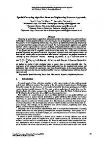
Fig. 1. A slice of the simulated 3-D brain image from MNI (z = 60). (a) True model. (b) Image corrupted with noise and INU artifact. (c) The corresponding bias field.
(a)
(b)
(c)
Fig. 2. Segmentation result for the MRI image of Fig. 1(b). (a) The segmentation using the proposed algorithm. (b) The recovered bias field. (c) The segmentation using the conventional FCM algorithm.
produced by multiplying the simulated MR image by a bias field recovered from an actual MR scan according to the image formation model of (1).4 Extra-cranial tissues were removed from all images prior to segmentation. For real data, this can be done using any of the techniques reported in the literature [32]–[36]. Fig. 1 shows a slice of the simulated MRI brain data, . The brain image of Fig. 1(a) was generated taken at based on a discrete anatomical normal brain model, and serves as the true model. The image of Fig. 1(b) was simulated from modality, ICBM the true model with the following settings: voxels), 3% protocol [29], slice thickness of 1 mm (1 noise level and 40% INU. Fig. 1(c) shows the actual bias field that produces the INU artifact. It was obtained by solving for (1), using the noise-free, INU artifact-free data and the noise-free, INU affected data, obtained also from MNI. The number of tissue classes in the segmentation was set to three, which corresponds to gray matter (GM), white matter (WM) and cerebrospinal fluid (CSF). Background pixels are ignored in the computation. For all the segmentation experiments, , , the default parameter values used are: number of spline intervals in the and dimensions, , maximum number of iterations . The algorithm usually converges in around 6–7 iterations. For the simulated 3-D MRI brain image of dimension 217 181 181 [row ( ) column ( ) depth ( )], the total computation time is around 1.5–2 min on a Pentium 4 2-GHz PC. A. Visual Evaluation Fig. 2(a) shows the segmented image. The segmentation can be observed to correspond well to the true model in Fig. 1(a). 4This was done by MNI. However, we have verified experimentally, through the computation of the actual bias field shown Fig. 1(c), that they actually used the multiplicative model of (1) in simulating the INU artifact.
(a)
(b)
Fig. 3. Segmentation result for the slice near the base of the brain (z = 35). (a) True model. (b) Segmented result.
Fig. 2(b) shows the recovered bias field, which resembles very closely the actual bias field of Fig. 1(c). In comparison, we also show in Fig. 2(c) the segmentation by the conventional FCM algorithm, whose accuracy is severely affected by noise and INU. The results clearly indicate that the proposed algorithm is able to compensate for noise and INU artifact in the input image. Figs. 3 and 4 show the ground truth and the segmentation re(near the base of the brain) and sult for slices taken at (near the top of the skull), respectively. Although they are more difficult to segment than slices from the center of the brain, the results show that accurate segmentation can still be achieved. Fig. 5(a) shows an across-slice view of the actual bias field, , for the same data set. Fig. 5(b) shows the estitaken at mated bias field taken at the same location. As can be seen, the estimated bias field has captured accurately the intensity inhomogeneity across slices without exhibiting between-slice discontinuity in spite of the modeling of the 3-D bias field by a stack of 2-D spline surfaces. The second regularizing term of
LIEW AND YAN: ADAPTIVE SPATIAL FUZZY CLUSTERING ALGORITHM FOR 3-D MR IMAGE SEGMENTATION
(a)
(b)
Fig. 4. Segmentation result for the slice near the top of the skull (z (a) True model. (b) Segmented result.
1071
= 140).
Fig. 6. Mean intensity value of WM as a function of z -coordinate, from the base of the brain to the top of the brain. The dashed line is for the uncorrected ); the solid line is for the INU corrected data. The dotted line data ( is for the data with no INU.
INU = 40%
(a)
(b)
TABLE I MISCLASSIFICATION RATE FOR DIFFERENT INU CORRECTION SEGMENTATION METHODS AT DIFFERENT INU LEVEL
AND
= 110
Fig. 5. (a) Actual, and (b) computed bias field for y . The x coordinate increases from left to right and the z coordinate increases from bottom to top.
(20) has successfully constrained the estimated 3-D field to be smooth in the direction. To show the effectiveness of the bias correction method, Fig. 6 shows the mean intensity value of the WM from the base of the brain to the top of the brain. The uncorrected data with 40% INU (dashed line) shows significant variation in intensity value whereas the INU corrected data (solid line) has a more uniform WM intensity value. For comparison, the WM mean intensity value for the data with no INU (dotted line) is also shown. Besides a constant offset, the remarkable similarity in the shape of the two curves indicates that INU has been correctly compensated for. Note that the mean intensity value for the data with no INU is not a constant straight line. This is due largely to partial volume effect, where a voxel is partially shared by two or more tissue types. This phenomenon is particularly noticeable at the two extremes of the brain, where boundaries between tissue types become less defined. The proposed algorithm is also able to correctly take that into account as reflected in the closely matched shape around the two ends of the curve. B. Quantitative Evaluation For a quantitative evaluation of the performance of the algorithm, we compute the misclassification rate (MCR) for the segmentation of the simulated MRI data ( weighted, 1 voxels, 3% noise) with varying level of INU inhomogeneity (i.e., 0% INU, 20% INU, 40% INU). The MCR is defined as the number of pixels misclassified by the algorithm divided by the total number of pixels in the image. For comparison, we quote the MCR of the different INU estimation algorithms as reported in [15]. The results are presented in Table I. FCM denotes the
conventional FCM algorithm. FM -AFCM and TM-AFCM denote the full multigrid adaptive FCM algorithm and the truncated multigrid adaptive FCM algorithm, respectively [15]. EM1 and EM2 denote the unsupervised EM algorithm for finite Gaussian mixture models, where EM1 refers to the standard model and EM2 refers to the model where variances and mixture coefficients of the Gaussian components are assumed equal [30]. AMRF denotes the adaptive Markov random field algorithm [31], [32]. MNI-FCM denotes the method where inhomogeneity correction technique [9] from MNI is the applied first, followed by FCM segmentation. From Table I, we see that the MCR generally increases with an increase in the INU level. Also, our method has significantly better performance than other methods and is more robust to increased inhomogeneity. For the 40% INU level, our method shows an improvement of 58% over the FCM method, 24% over the FM -AFCM method, 22% over the TM-AFCM method, 72% over the EM1 method, 60% over the EM2 method, 44% over the AMRF method and 32% over the MNI-FCM method. We also compare our results with the results obtained by the EM-MRF algorithm of Leemput et al. [39], [40].5 In the EM-MRF algorithm, the MRI brain tissue classes are modeled 5Downloaded from loads/ems/ems.html
http://bilbo.esat.kuleuven.ac.be/web-pages/down-
1072
IEEE TRANSACTIONS ON MEDICAL IMAGING, VOL. 22, NO. 9, SEPTEMBER 2003
TABLE II COMPARISON BETWEEN OUR ALGORITHM AND THE EM-MRF ALGORITHM: IN TERMS OF OVERLAP METRIC (IN %) FOR DIFFERENT TISSUE CLASS, AND THE MCR (IN %), FOR DIFFERENT INU LEVEL. “NO MRF” DENOTES THE EM-MRF ALGORITHM WITHOUT MRF REGULARIZATION, “WITH MRF” DENOTES THE EM-MRF ALGORITHM WITH MRF REGULARIZATION
as finite Gaussian mixtures with Markov random field regularization and digital brain atlas initialization, and the bias field is modeled as a fourth order least square polynomial fit. For the EM-MRF method, we calculated both the MCR and the overlap , metric [41]. The overlap metric is define as denotes the number of voxels assigned to class where by both the ground truth and the algorithm, and denote the number of voxels assigned to class by the algorithm and the ground truth, respectively, for the three tissue classes. The overlap metric attains the value of one if both segmentations are in full agreement and zero if there is no overlap at all. We run both our algorithm and the EM-MRF algorithm on the three simulated MRI datasets. The comparison results are tabulated in Table II. For the EM-MRF algorithm, we used two different settings: one with MRF regularization and the other one without MRF regularization. The results show that our algorithm has performed well over all three tissue types compared to the EM-MRF algorithm, even though the EM-MRF algorithm uses a prior classification derived from a digital brain atlas that contains spatially varying prior probability maps for the location of CSF, GM, and WM. It is also remarkable that the performance of our method, even at 40% INU, is still better than the FCM method at 0% INU. Our method has a slightly inferior performance at 0% INU than at 20% INU. This is due to the additional degree of freedom associated with the bias field. This effect is also observed in the MNI-FCM method. One can easily reduce the error by increasing if the amount of inhomogeneity is known to be low. It is interesting to note that at 0% INU, our method, with the additional degree of freedom, still performs better than the FCM method. This is due to the spatial continuity constraint in our algorithm, which smoothes out noise and reduces classification ambiguity. To see the advantage of incorporating the spatial continuity constraint, we set the bias field in our algorithm to zero and carried out the segmentation on 0% INU data with just the spatial continuity constraint. The MCR for this case is 3.474%, an improvement of over 13% over the FCM method. If we just have the bias field correction but not the spatial continuity constraint, we get an MCR of 4.003% at 0% INU, which is inferior to the FCM method, as expected. The difference, however, is small, indicating that our method performs well on images of varying inhomogeneity, without the need for tedious adjustment of the regularizing parameters. The advantage of having a noise smoothing property is also observed in the AMRF method at 0% INU, which has a slightly better performance than the FCM method.
TABLE III MISCLASSIFICATION RATE FOR THE SAME DATASET REFORMATTED DIFFERENT SLICE PLANES
AT
TABLE IV MISCLASSIFICATION RATE AS A FUNCTION OF REGULARIZATION PARAMETER AND THE NUMBER OF SPLINE INTERVALS nx WITH = 2 10
2
TABLE V MISCLASSIFICATION RATE AS A FUNCTION OF REGULARIZATION PARAMETERS AND WITH nx = 2
As a mean of quantitatively validating the two-stage approach for 3-D bias field estimation for slices taken at different planes, we computed the MCR for the same dataset (which is originally in transverse slices) reformatted as coronal slices and sagittal slices. The results are presented in Table III. The results show that the two-stage approach for estimating the 3-D bias field is insensitive to the slice plane. We remark that if the bias field estimation is required to be totally invariant to the slice plane, one possible approach is to compute a bias field for each slice plane, and then average the three bias fields to get the slice-plane invariant bias field in each iteration. C. Variation of Algorithmic Parameters Table IV shows the MCR after applying the proposed voxels, ASFCM algorithm to the simulated data set (1 3% noise, and 40% INU) when varying the regularizing
LIEW AND YAN: ADAPTIVE SPATIAL FUZZY CLUSTERING ALGORITHM FOR 3-D MR IMAGE SEGMENTATION
1073
(a)
(b)
(c)
(d)
(e)
(f)
Fig. 7. Segmentation of real MRI image. (a) Original image. (b) INU corrected image. (c) Proposed ASFCM segmentation. (d) FCM segmentation. (e) Estimated bias field. (f) Intensity histogram before (dashed line) and after (solid line) INU correction.
(a)
(b)
(c)
(d)
(e)
(f)
Fig. 8. Segmentation of another real MRI image. (a) Original image. (b) INU corrected image. (c) Proposed ASFCM segmentation. (d) FCM segmentation. (e) Estimated bias field. (f) Intensity histogram before (dashed line) and after (solid line) INU correction.
parameter
and the number of spline intervals, while setting . As can be seen, the algorithm is insensitive to both parameters. The bias field can adequately be modeled by -spline surfaces with very few intervals since the bias field is known a priori to be smooth. We observe that fewer spline intervals generally give better results. This can be explained by the fewer degree-of-freedom, which implicitly imposes a strong constraint on the smoothness of the spline surface. Nevertheless, if the bias field were known to have large spatial variation, more spline intervals would be needed to ensure an would suffice adequate fit. Even so, in most cases. Table V shows the MCR when varying and , while setting the number of spline intervals to two. Again,
the proposed algorithm is insensitive to the parameter settings. Finally, we observe that the different parameter combinations in Tables IV and V all have an MCR of less than the seven other methods we compare in Table I (see last column in Table I), and even the FCM at 0% INU, indicating the robustness and efficacy of our algorithm. D. Performance on Actual MRI Data Figs. 7 and 8 show one slice of the segmentation results for two real -weighted MR images using the proposed algorithm. Figs. 7(a) and 8(a) are the original images. Figs. 7(b) and 8(b) are the INU corrected images. The INU artifact has largely been suppressed and one can see a fairly uniform image compared
1074
IEEE TRANSACTIONS ON MEDICAL IMAGING, VOL. 22, NO. 9, SEPTEMBER 2003
to the original image. Figs. 7(c) and 8(c) show the segmentations using our method. Figs. 7(d) and 8(d) show the segmentations using the FCM algorithm. Visual inspection shows that our method produces better segmentations than the FCM algorithm. In particular, the GM and WM in the top region of both images can be better separated by our method. Figs. 7(e) and 8(e) show the estimated bias fields. The bias field has successfully captured the different shading in the original images. Figs. 7(f) and 8(f) show the intensity histogram of the slices before and after INU correction. One can see that there is less spread in the histogram after INU correction. Also, the two prominent peaks, which correspond to the GM and WM are sharper and better resolved in the INU corrected images. VI. CONCLUSION We have presented an adaptive spatial FCM segmentation algorithm that takes into account a local spatial continuity constraint, as well as the suppression of the INU artifact in 3-D MR images. The algorithm employs a novel dissimilarity index that considers the local influence of neighboring pixels in an adaptive manner. If the neighborhood window is in a nonhomogeneous region, the influence of the neighboring voxels on the center voxel is suppressed; otherwise, the center voxel is smoothed by its neighboring voxels during membership and cluster centroid computation. To suppress the INU artifact, a multiplicative MR image formation model is used. The estimation of the 3-D multiplicative bias field is formulated as the estimation of a stack of 2-D smoothing spline surfaces, with continuity enforced across slices, minimizing the 3-D residual signal between the actual data and a piecewise constant FCM solution. The -spline coefficients of the spline surfaces are obtained by a computationally efficient two-stage algorithm. Extensive experiment results and comparative studies with several existing methods on the segmentation of both simulated and real MR brain images illustrate the effectiveness and robustness of our algorithm. ACKNOWLEDGMENT The authors would like to thanks the anonymous reviewers whose comments greatly improved the paper. REFERENCES [1] J. C. Bezdek, Pattern Recognition with Fuzzy Objective Function Algorithms. New York: Plenum, 1981. [2] J. C. Bezdek, L. O. Hall, and L. P. Clark, “Review of MR image segmentation techniques using pattern recognition,” Med. Phys., vol. 20, pp. 1033–1048, 1993. [3] M. Singh, P. Patel, D. Khosla, and T. Kim, “Segmentation of functional MRI by K-means clustering,” IEEE Trans. Nucl. Sci., vol. 43, pp. 2030–2036, June 1996. [4] L. O. Hall, A. M. Bensaid, L. P. Clarke, R. P. Velthuizen, M. S. Silbiger, and J. C. Bezdek, “A comparison of neural network and fuzzy clustering techniques in segmenting magnetic resonance images of the brain,” IEEE Trans. Neural Networks, vol. 3, pp. 672–682, Sept. 1992. [5] A. Simmons, P. S. Tofts, G. J. Barker, and S. R. Arridge, “Sources of intensity nonuniformity in spin echo images at 1.5 T,” Magn. Reson. Med., vol. 32, pp. 121–128, 1994. [6] L. G. Nyul, J. K. Udupa, and X. Zhang, “New variants of a method of MRI scale standardization,” IEEE Trans. Med. Imag., vol. 19, pp. 143–150, Feb 2000.
[7] C. R. Meyer, P. H. Bland, and J. Pipe, “Retrospective correction of intensity inhomogeneities in MRI,” IEEE Trans. Med. Imag., vol. 12, pp. 36–41, Mar. 1995. [8] B. M. Dawant, A. P. Zijdenbos, and R. A. Margolin, “Correction of intensity variations in MR images for computer-aided tissue classification,” IEEE Trans. Med. Imag., vol. 12, pp. 770–781, Dec 1993. [9] J. G. Sled, A. P. Zijdenbos, and A. C. Evans, “A nonparametric method for automatic correction of intensity nonuniformity in MRI data,” IEEE Trans. Med. Imag., vol. 17, pp. 87–97, Feb 1998. [10] W. M. Wells III, W. E. L. Grimson, R. Kikinis, and F. A. Jolesz, “Adaptive segmentation of MRI data,” IEEE Trans. Med. Imag., vol. 15, pp. 429–442, Aug 1996. [11] M. Tincher, C. R. Meyer, R. Gupta, and D. M. Williams, “Polynomial modeling and reduction of RF body coil spatial inhomogeneity in MRI,” IEEE Trans. Med. Imag., vol. 12, pp. 361–365, June 1993. [12] B. H. Brinkmann, A. Manduca, and R. A. Robb, “Optimized homomorphic unsharp masking for MR grayscale inhomogeneity correction,” IEEE Trans. Med. Imag., vol. 17, pp. 161–171, Apr. 1998. [13] B. Johnston, M. S. Aitkins, B. Mackiewich, and M. Anderson, “Segmentation of multiple sclerosis lesions in intensity corrected multispectral MRI,” IEEE Trans. Med. Imag., vol. 15, pp. 154–169, Apr. 1996. [14] M. Styner, C. Brechbuhler, G. Szekely, and G. Gerig, “Parametric estimate of intensity inhomogeneities applied to MRI,” IEEE Trans. Med. Imag., vol. 9, pp. 153–165, Mar. 2000. [15] D. L. Pham and J. L. Prince, “Adaptive fuzzy segmentation of magnetic resonance images,” IEEE Trans. Med. Imag., vol. 18, pp. 737–751, Sept. 1999. [16] J. O. Eklundh, H. Yamamoto, and A. Rosenfeld, “A relaxation method for multi-spectral pixel classification,” IEEE Trans. Pattern Anal. Machine Intell., vol. PAMI-2, pp. 72–75, 1980. [17] J. Y. Hsiao and A. Sawchuk, “Supervised textured image segmentation using feature smoothing and probabilistic relaxation techniques,” IEEE Trans. Pattern Anal. Machine Intell., vol. PAMI-11, pp. 1279–1292, 1989. , “Unsupervised textured image segmentation using feature [18] smoothing and probabilistic relaxation techniques,” Comput. Vis., Graph., Image Processing, vol. 48, pp. 1–21, 1989. [19] Y. A. Tolias and S. M. Panas, “Image segmentation by a fuzzy clustering algorithm using adaptive spatially constrained membership functions,” IEEE Trans. Syst., Man, Cybern. A, vol. 28, pp. 359–369, May 1998. [20] A. W. C. Liew, S. H. Leung, and W. H. Lau, “Fuzzy image clustering incorporating spatial continuity,” Inst. Elect. Eng. Proc.-Vision, Image and Signal Processing, vol. 147, pp. 185–192, Apr. 2000. [21] J. K. Udupa and S. Samarasekera, “Fuzzy connectedness and object definition: Theory, algorithms and applicationa in image segmentation,” Graph. Models Image Process., vol. 58, pp. 246–261, 1996. [22] J. K. Udupa, L. Wei, S. Samarasekera, Y. Miki, M. A. van Buchem, and R. I. Grossman, “Multiple sclerosis lesion quantification using fuzzy connectedness principles,” IEEE Trans. Med. Imag., vol. 16, pp. 598–609, Oct. 1997. [23] P. Dierckx, Curve and Surface Fitting with Splines. Oxford, U.K.: Oxford Univ., 1993, Monographs on Numerical Analysis. [24] W. H. Press, S. A. Teukolsky, W. T. Vetterling, and B. P. Flannery, Numerical Recipes in C, 2nd ed. Cambridge, U.K.: Cambridge Univ. Press, 1992. [25] McGill Univ., Quebec, ON, Canada.. [Online]. Available: Available: http://www.bic.mni.mcgill.ca/brainweb [26] C. A. Cocosco, V. Kollokian, R. K. S. Kwan, and A. C. Evans, “BrainWeb: Online interface to a 3D MRI simulated brain database,” NeuroImage, pt. 2/4, S425, vol. 5, no. 4, 1997. [27] D. L. Collins, A. P. Zijdenbos, V. Kollokian, J. G. Sled, N. J. Kabani, C. J. Holmes, and A. C. Evans, “Design and construction of a realistic digital brain phantom,” IEEE Trans. Med. Imag., vol. 17, pp. 463–468, June 1998. [28] R. K. S. Kwan, A. C. Evans, and G. B. Pike, “An extensible MRI simulator for post-processing evaluation,” in Lecture Notes in Computer Science. Berlin, Germany: Springer-Verlag, 1996, vol. 1131, Proceedings Visualization in Biomedical Computing (VBC’96), pp. 135–140. [29] Univ. California, Int. Consortium Brain Mapping (ICBM), Lab. Neuro Imag., Quebec, ON, Canada., Los Angeles, CA. [Online]. Available: http://www.loni.ucla.edu/ICBM/ [30] Z. Liang, R. J. Jaszczak, and R. E. Coleman, “Parameter estimation of finite mixtures using the EM algorithm and information criteria with application to medical image processing,” IEEE Trans. Nucl. Sci., vol. 39, pp. 1126–1133, Aug. 1992.
LIEW AND YAN: ADAPTIVE SPATIAL FUZZY CLUSTERING ALGORITHM FOR 3-D MR IMAGE SEGMENTATION
[31] M. X. H. Yan and J. S. Karp, “An adaptive Bayesian approach to threedimensional MR brain segmentation,” in Proc. Information Processing and Medical Imaging (IPMI’95), 1995, pp. 201–213. [32] A. F. Goldszal, C. Davatzikos, D. L. Pham, M. X. H. Yan, R. N. Bryan, and S. M. Resnick, “An image processing system for qualitative and quantitative volumetric analysis of brain images,” J. Comput. Assist. Tomogr., vol. 22, pp. 827–837, 1998. [33] B. Mackiewich, “Intracranial boundary detection and radio frequency correction in magnetic resonance images,” Master’s, Simon Fraser Univ., Comput. Sci. Dept., Burnaby, BC, Canada, 1995. [34] S. Sandor and R. Leahy, “Toward automated labeling of the cerebral cortex using a deformable atlas,” in Proc. Information Processing and Medical Imaging (IPMI’95), 1995, pp. 127–138. [35] T. Kapur, W. E. L. Grimson, W. M. Wells III, and R. Kikinis, “Segmentation of brain tissue from magnetic resonance images,” Med. Image Anal., vol. 1, pp. 109–127, 1996. [36] F. Kruggel and G. Lohman, “Automatic adaption of the stereotactical coordinate system in brain MRI datasets,” in Proc. Information Processing and Medical Imaging (IPMI’97), 1997, pp. 471–476.
1075
[37] H. E. Cline, W. E. Lorensen, R. Kikinis, and F. Jolesz, “Three dimensional segmentation of MR images of the head using probability and connectivity,” J. Comput. Assist. Tomogr., vol. 14, pp. 1037–1045, 1990. [38] M. E. Brummer, R. M. Mersereau, R. L. Eisner, and R. R. J. Lewine, “Automatic detection of brain contours in MRI data sets,” IEEE Trans. Med. Imag., vol. 12, pp. 153–166, June 1993. [39] K. V. Leemput, F. Maes, D. Vandermeulen, and P. Suetens, “Automated model-based bias field correction of MR images of the brain,” IEEE Trans. Med. Imag., vol. 18, pp. 885–896, Oct. 1999. , “Automated model-based tissue classification of MR images of [40] the brain,” IEEE Trans. Med. Imag., vol. 18, pp. 897–908, Oct. 1999. [41] A. Zijdenbos, B. M. Dawant, R. A. Margolin, and A. C. Palmer, “Morphometric analysis of white matter lesions in MR images: Method and validation,” IEEE Trans. Med. Imag., vol. 13, pp. 716–724, Dec. 1994.