An algebraic method for solving central force problems T. H. Cookea) and J. L. Wood School of Physics, Georgia Institute of Technology, Atlanta, Georgia 30332-0430
共Received 23 July 2001; accepted 9 May 2002兲 A simple algebraic method, which is as easy to use as the angular momentum algebra, is demonstrated as a pedagogical way to solve certain central force problems exactly. Solutions for the hydrogen atom and the three-dimensional isotropic harmonic oscillator are presented together with a discussion of the limits of the method. © 2002 American Association of Physics Teachers. 关DOI: 10.1119/1.1491262兴
closed algebra. Thus, r a⫹b⫺1 must be equal to r a , whence b⫽1 and 关 r a ,rp 兴 ⫽iaបr a . Similarly, we obtain for the other commutator brackets,
I. INTRODUCTION The central force problem, H 兩 Elm 典 ⫽E 兩 Elm 典 ,
共1兲
关 r a ,r 2⫺a p 2 兴 ⫽a 共 a⫺1 兲 ប 2 ⫹2iaបrp,
where
关 rp,r
p 2 l 共 l⫹1 兲 ប 2 ⫹ ⫹V 共 r 兲 , H⫽ 2m 2mr 2
共2兲
and p⫽p r is a familiar one in quantum physics. It covers the Coulomb potential 共Fig. 1兲, which describes the hydrogen atom, as well as the three-dimensional isotropic harmonic oscillator potential 共Fig. 2兲, which is used as an approximation to the strong force independent–particle mean field in nuclei. Finding exact solutions to these problems by differential methods is tedious. We outline an algebraic way1 of solving for the energy eigenvalues and eigenfunctions that is more elegant than the traditional differential methods, and also explore the limits of this method.
p ,
共10兲 共11兲
where c⫽2⫺a is chosen so that the algebra closes. Note that these brackets do not depend in any way on the choice of a potential. Indeed, we choose the remaining degree of freedom, a, to fit our algebra to the potentials we solve. We introduce the change of variables, viz., V 1 ⫽r a ,
共12兲
1 V 2 ⫽ 关 rp⫺ 21 i 共 a⫺1 兲 ប 兴 , a
共13兲
V 3⫽
A well-known example of an algebraic solution to a standard quantum mechanical problem is the solution to the angular momentum problem, L 2 兩 典 ⫽ 兩 典 ,
共3兲
L z兩 典 ⫽ 兩 典 ,
共4兲
which uses the commutator brackets 关 L x ,L y 兴 ⫽iបL z ,
共5兲
关 L y ,L z 兴 ⫽iបL x ,
共6兲
关 L z ,L x 兴 ⫽iបL y ,
共7兲
1 2⫺a 2 r p . a2
共14兲
and yields ⫽l(l⫹1)ប , ⫽mប (m⫽l,l⫺1,...,1,0,⫺1,..., ⫺l). These commutator brackets, or Lie products, define the Lie algebra2 so共3兲. The algebraic solution to 共1兲 can be achieved using the commutator bracket, 关 r,p m 兴 ⫽iបmp m⫺1 ,
共8兲 a
关 V 2 ,V 3 兴 ⫽iបV 3 ,
共16兲
关 V 3 ,V 1 兴 ⫽⫺2iបV 2 .
共17兲
共18兲
Therefore, from Eqs. 共16兲 and 共18兲 we obtain ⫺1 关 V 2 , 共 V 3 ⫹ V ⫺1 1 兲兴 ⫽iប 共 V 3 ⫹ V 1 兲 ,
共19兲
where is a constant or any operator that commutes with V 1 , V 2 , and V 3 . That is, the algebra of Eqs. 共15兲–共17兲 is unchanged by the replacement of V 3 with V 3 ⫹ V ⫺1 1 . With one last linear combination 共extension兲 of the algebra, viz.,
b
共9兲
Just as L x , L y , and L z form the closed algebra of Eqs. 共5兲– 共7兲, we want the Lie products of r a , r b p, and r c p 2 to form a
共15兲
⫺1 关 V 2 ,V ⫺1 1 兴 ⫽iបV 1 .
and the Lie products that result for the operators r , r p, and r c p 2 . 关We only consider powers of p up to p 2 because that is the highest power of p in Eq. 共1兲.兴 From Eq. 共8兲 we obtain 关 r a ,r b p 兴 ⫽r b 关 r a , p 兴 ⫽r b 共 iបar a⫺1 兲 ⫽iបar a⫹b⫺1 .
关 V 1 ,V 2 兴 ⫽iបV 1 ,
A subtle and key extension of this algebraic structure is realized3 by noting that a can take on both positive and negative values in Eq. 共12兲, and therefore that r ⫺a ⫽V ⫺1 1 yields, from Eqs. 共9兲 and 共13兲,
2
Am. J. Phys. 70 共9兲, September 2002
2⫺a 2
The commutator brackets, Eqs. 共9兲, 共10兲, and 共11兲, can now be written as
II. BUILDING THE ALGEBRA
945
p 兴 ⫽iបar
2⫺a 2
T 1 ⫽ 21 共 V 3 ⫹ V ⫺1 1 ⫺V 1 兲 ,
共20兲
T 2 ⫽V 2 ,
共21兲
T 3 ⫽ 21 共 V 3 ⫹ V ⫺1 1 ⫹V 1 兲 ,
共22兲
we obtain the commutator algebra,
http://ojps.aip.org/ajp/
关 T 1 ,T 2 兴 ⫽⫺iបT 3 , © 2002 American Association of Physics Teachers
共23兲 945
where ␥ ⫽⫹1 for so共3兲 and ␥ ⫽⫺1 for so共2,1兲. Using these equations enables us to translate much of our knowledge of so共3兲 into so共2,1兲. For example, the raising and lowering operators are T ⫾ ⫽T 1 ⫾iT 2 , and produce 关 T ⫹ ,T ⫺ 兴 ⫽2 ␥ បT 3 ,
共29兲
关 T 3 ,T ⫾ 兴 ⫽⫾បT ⫾ ,
共30兲
T
2
⫽ ␥ 共 T 21 ⫹T 22 兲 ⫹T 23 ⫽ ␥ T ⫹ T ⫺ ⫹T 23 ⫺បT 3 ⫽ ␥ T ⫺ T ⫹ ⫹T 23 ⫹បT 3 ,
关 T 2 ,T 兴 ⫽0,
共31兲
⫽1,2,3.
共32兲 2
Simultaneous eigenkets of T and T 3 exist and obey
Fig. 1. The hydrogen atom–the Coulomb potential is the dotted line, the ‘‘centrifugal’’ potential is the dashed line, and the total potential is the solid line.
T 2 兩 Qq 典 ⫽Q 兩 Qq 典 ,
共33兲
T 3 兩 Qq 典 ⫽q 兩 Qq 典 ,
共34兲
T 3 T ⫾ 兩 Qq 典 ⫽ 共 q⫾ប 兲 T ⫾ 兩 Qq 典 .
共35兲
关 T 2 ,T 3 兴 ⫽iបT 1 ,
共24兲
Thus the T ⫾ operators perform ladder operations on the eigenvectors of T 3 , and therefore the eigenvalue– eigenvector spectrum of T 3 is obtained. So, to find the constraints on the eigenvalues, we consider
关 T 3 ,T 1 兴 ⫽iបT 2 .
共25兲
具 Qq 兩 共 T 2 ⫺T 23 兲 兩 Qq 典 ⫽Q⫺q 2 ,
These are reminiscent of the angular momentum commutator brackets mentioned in Eqs. 共5兲–共7兲. Equations 共23兲–共25兲 are identical to Eqs. 共5兲–共7兲 except for the sign difference between Eqs. 共5兲 and 共23兲. The Lie algebra described by L x , L y , and L z is so共3兲, whereas the algebra described by T 1 , T 2 , and T 3 is so共2,1兲. We learn a great deal about this algebra by comparing it with our knowledge of angular momentum.
␥ ⫽ 具 Qq 兩 共 T ⫹ T ⫺ ⫹T ⫺ T ⫹ 兲 兩 Qq 典 . 2 By rewriting Eq. 共36兲 using T ⫹ 兩 Qq 典 ⫽ 兩 典 ,
共37兲
T ⫺ 兩 Qq 典 ⫽ 兩 典 ,
共38兲
4
we obtain 1 2
III. A COMPARISON OF so„3… AND so„2,1… To compare the algebras so共2,1兲 and so共3兲, we write them in the condensed form 关 T 1 ,T 2 兴 ⫽i ␥ បT 3 ,
共26兲
关 T 2 ,T 3 兴 ⫽iបT 1 ,
共27兲
关 T 3 ,T 1 兴 ⫽iបT 2 ,
共28兲
共36兲
具 Qq 兩 T 共 T ⫹ T ⫺ ⫹T ⫺ T ⫹ 兲 兩 Qq 典 ⫽ 具 兩 典 ⫹ 具 兩 典 ⭓0, 共39兲
which means, for ␥ ⫽⫹1, Q⫺q 2 ⭓0,
共40兲
q⭐ 冑Q.
共41兲
Equation 共41兲 is the result we expect for so共3兲. The eigenvalues of T 3 (L z ) are bounded above and below, creating a range of values for q(m l ). 共Moreover, from these bounds it follows that m l ⫽l,l⫺1,...,1,0,⫺1,..., l.兲 However, for ␥ ⫽⫺1, Q⫺q 2 ⭐0,
共42兲
q⭓ 冑Q.
共43兲
Either q has a lower bound or an upper bound, but not both. 关Because of the infinite nature of the eigenvalues, so共2,1兲 is called a noncompact algebra.兴 We choose for q to have a lower bound; the motivation for this choice will become evident later. We define the lowest eigenstate as T ⫺ 兩 Qq 0 典 ⫽0,
共44兲
and find T 2 兩 Qq 0 典 ⫽ 共 ⫺T ⫹ T ⫺ ⫹T 23 ⫺បT 3 兲 兩 Qq 0 典 ⫽ 共 q 20 ⫺q 0 ប 兲 兩 Qq 0 典 ⫽q 0 共 q 0 ⫺ប 兲 兩 Qq 0 典 .
共45兲
5
Fig. 2. The 3D harmonic oscillator–the oscillator potential is the dotted line, the ‘‘centrifugal’’ potential is the dashed line, and the total potential is the solid line. 946
Am. J. Phys., Vol. 70, No. 9, September 2002
Just as the irreducible representations of so共3兲 are labeled by l and the eigenvalues of L 2 are l(l⫹1), so the irreducible representations of so共2,1兲 are labeled by q 0 , and the eigenvalues of T 2 are q 0 (q 0 ⫺ប). The only difference between T. H. Cooke and J. L. Wood
946
the irreps of the two groups is that the irreducible representations of so共3兲 consist of a finite number of states, whereas the irreducible representations of so共2,1兲 consist of an infinite number of states. To illuminate the nature of q 0 , consider T
2
⫽⫺T 21 ⫺T 22 ⫹T 23 ⫽ 共 T 3 ⫺T 1 兲共 T 3 ⫹T 1 兲 ⫺ 关 T 3 ,T 1 兴 ⫺T 22 2 ⫽V 1 共 V 3 ⫹ V ⫺1 1 兲 ⫺iបV 2 ⫺V 2 .
Then, using V 22 ⫽
冉
冋
a⫺1 1 2 2 ប 2 r p ⫺iaបr p⫺ a 2
共46兲
冊册 2
共47兲
关from Eqs. 共8兲 and 共13兲兴, and Eqs. 共12兲, 共13兲, and 共14兲, we can simplify Eq. 共46兲 to T 2⫽ ⫹
ប2 共 1⫺a 2 兲 . 4a 2
具 Qq 0 兩 T 2 兩 Qq 0 典 ⫽q 0 共 q 0 ⫺ប 兲 ,
冋
q 20 ⫺q 0 ប⫺ ⫹
q 0⫽
冉 冑
ប 1⫾ 2
共49兲
册
ប2 共 1⫺a 2 兲 ⫽0, 4a 2
which implies that
r
冋 冉冊
a r d n共 r 兲 ⫹ ⫺ dr ប ␣
共50兲
冊
4 1 ⫹ . ប2 a2
共51兲
To find the ground state wave function, consider 共 T ⫺ ⫺T 3 兲 兩 Qq 0 典 ⫽⫺q 0 兩 Qq 0 典 .
共52兲
共 V 1 ⫹iV 2 ⫺q 0 兲 兩 Qq 0 典 ⫽0,
which simplifies to
册
ir p ប a⫺1 ⫹ ⫺q 0 兩 Qq 0 典 ⫽0. a 2 a
冋冉冊
a r d 0共 r 兲 ⫹ dr ប ␣
a
⫹
册
a⫺1 aq 0 ⫺ 0 共 r 兲 ⫽0, 2 ប
a
0 共 r 兲 ⫽Ar C e ⫺ 共 1/ប 兲共 r/ ␣ 兲 ,
共54兲
共55兲
共56兲
where C⫽aq 0 ប ⫺1 ⫺1/2(a⫺1). The substitution of q 0 from Eq. 共51兲 gives
冋 冑
1 1⫾ 2
册
4a 2 ⫹1 . ប2
共57兲
The excited state wave functions can be obtained using 关 T ⫹ ⫺ 共 T 3 ⫺q n 兲兴 n 共 r 兲 ⫽ n⫹1 n⫹1 共 r 兲 , 947
共60兲
where n (r) is the radial portion of the wave function that solves the original three-dimensional problem, and ⌿(r) is the wave function that solves the simplified one-dimensional radial problem stated in Eq. 共2兲. V. THE LIMITS OF so„2,1… AS APPLIED TO CENTRAL FORCE PROBLEMS All of the problems under consideration are based upon the connection between the so共2,1兲 operator T 3 and the Hamiltonian operator, as follows: 共 T 3 ⫺q n 兲 ⫽ ␣ r  共 H⫺E 兲 .
共61兲
冉
Am. J. Phys., Vol. 70, No. 9, September 2002
冊
1 1 2⫺a 2 r p ⫹ a ⫹r a ⫺q n 2 a2 r ⫽␣r
冋
册
p 2 l 共 l⫹1 兲 ប 2 ⫹ ⫹V 共 r 兲 ⫺E . 2m 2mr 2
共62兲
Immediately the terms in p 2 can be equated, and the result is ␣ ⫽ma ⫺2 and  ⫽2⫺a. Therefore, Eq. 共62兲 reduces to
where ␣ permits a scaling of the position coordinate. It directly follows that Eq. 共55兲 is separable, and thus ⌿ 0 (r) can be written as
C⫽
共59兲
n 共 r 兲 ⬅r n 共 r 兲 ,
共53兲
If we express Eq. 共54兲 in the position representation 关r→ ␣ ⫺1 r,p→⫺iប ␣ d/dr, 兩 Qq 典 →⌿ 0 (r)兴, we obtain the differential equation r
册
a⫺1 aq n ⫹ n共 r 兲 2 ប
The actual calculation of the excited state wave functions 共and of their normalization constants兲 is left as an exercise for the reader. Note that we have proceeded thus far by treating Eq. 共2兲 as a one-dimensional Hamiltonian. However, because radial integrals have an extra factor of r 2 compared with one-dimensional integrals, the three-dimensional wave functions are related to the one-dimensional wave functions we have found, viz.,
Using T ⫺ ⫽T 1 ⫺iT 2 and Eqs. 共20兲, 共21兲, 共22兲, we obtain
r a⫹
⫹
If we expand each side of Eq. 共61兲 and use Eqs. 共20兲, 共21兲, and 共22兲, we obtain
IV. WAVE FUNCTIONS
冋
a
⫽ n⫹1 n⫹1 共 r 兲 .
共48兲
From
we obtain
where n is a normalization constant and q n ⫽q 0 ⫹n r ប. Through a process similar to that leading from Eqs. 共52兲 to 共55兲, we write Eq. 共58兲 as
共58兲
冉
冊
l 共 l⫹1 兲 ប 2 r 2a a m m 1 ⫺ ⫹ ⫺r q n ⫺ 2 r 2 V 共 r 兲 ⫹ 2 r 2 E⫽0. 2 2 a 2 a a 共63兲 We can make a power series expansion of r 2 V(r) in r, but the only terms with nonzero coefficients will be terms of the same powers of r that we see in Eq. 共63兲, except for an r 2 term 共we do not wish to build the energy E into our potential兲. Thus, by inspection we write r 2 V 共 r 兲 ⫽A⫹Br 2a ⫹Dr a .
共64兲
If we substitute Eq. 共64兲 into Eq. 共63兲, we find
冉
冊冉
冊
1 m l 共 l⫹1 兲 ប 2 m 1 ⫺ ⫺ 2 A ⫹ ⫺ 2 B r 2a 2 2 a a 2 a
冉
⫺ q 0⫹
冊
m m 2 a 2 D r ⫹ 2 r E⫽0. a a
共65兲
It is impossible for the above equality to hold for all values of a without E being identically zero. However, for certain choices of a, one of the other terms will cancel the r 2 E term. T. H. Cooke and J. L. Wood
947
The first term, having no r dependence at all, cannot provide this cancellation. This leads to two possible cases: a⫽1 and a⫽2. By rearranging Eq. 共64兲, viz., A ⫹Br 2a⫺2 ⫹Dr a⫺2 , r2
q⫽q 0 ⫹n r ប⫽ 共 l⫹1 兲 ប⫹n r ប⫽
␣⫽
we see that A⫽0 and a⫽1 gives the Coulomb potential and A⫽0 and a⫽2 gives the harmonic oscillator potential. Note that the only other possible nonrelativistic central force problems solvable with the so共2,1兲 algebra are the modified Coulomb potential 共where A⫽0兲, and the Davidson6 potential 关the three-dimensional 共3-D兲 harmonic oscillator with A⫽0兴.
Finally,
4 ⑀ 0ប 关共 l⫹1 兲 ⫹n r 兴 . e2
E⫽⫺
The energy eigenvalue equation for the hydrogen atom is
冋
册
p2 l 共 l⫹1 兲 ប 2 e2 ⫹ ⫺ ⫺E 兩 Elm l 典 ⫽0. 2 4 ⑀ 0r 2r2
共67兲
If we multiply through by ␣ r, we obtain
冋
册
␣ r p 2 ␣ e 2 ␣ l 共 l⫹1 兲 ប 2 ⫹ ⫺ ⫺ ␣ rE 兩 Elm l 典 ⫽0. 共68兲 2 4⑀0 2r
The substitution R for ␣ ⫺1 r and P for ␣ p in Eq. 共68兲 produces
冋
册
R P 2 e 2 ␣ l 共 l⫹1 兲 ប 2 ⫺ ⫺ ␣ 2 RE 兩 Elm l 典 ⫽0. ⫹ 2 4⑀0 2R
共69兲
By using Eqs. 共12兲, 共13兲, and 共14兲, we rewrite Eq. 共69兲 as
冋
册
e ␣ 1 2 V 3⫺ ⫹l 共 l⫹1 兲 ប 2 V ⫺1 1 ⫺2 ␣ V 1 E 兩 Elm l 典 ⫽0, 2 2⑀0 共70兲 2
where a⫽1 so that the powers of R match. If we examine Eq. 共70兲 closely, we see that three terms match the definition of T 3 in Eq. 共22兲. In fact, if
e4 1 . 2 2 2 32 ⑀ 0 ប 共 l⫹1⫹n r 兲 2
共80兲
Ry . n2
共81兲
Note that here the irreducible representations of so共2,1兲 consist of energy eigenstates of a particular angular momentum, and therefore each irreducible representation is labeled by a value of angular momentum. The raising and lowering operators, T ⫾ , change the energy eigenstate within a particular irreducible representation, but do not move between irreducible representations. In other words, we can use T ⫾ to change n, but it does not change l. Another interesting point is that the Hamiltonian does not commute with all of the elements of so共2,1兲; unlike so共3兲, so共2,1兲 is not a symmetry group of the hydrogen atom. Instead, because the Hamiltonian is simply related to one of the generators, so共2,1兲 is called a dynamical symmetry group of the hydrogen atom. We immediately write the wave functions using Eq. 共56兲, viz.,
0 共 r 兲 ⫽Ar C e ⫺r/ ␣ ប .
共82兲
If we substitute for ␣ from Eq. 共79兲, we obtain
0 共 r 兲 ⫽Ar C e ⫺ e
2 r/4 ⑀ ប 2 n 0
共83兲
,
which simplifies to
0 共 r 兲 ⫽Ar C e ⫺r/na 0 ,
共84兲
⫽l 共 l⫹1 兲 ប ,
共71兲
where a 0 is the Bohr radius. From Eqs. 共57兲 and 共71兲 we calculate
2 ␣ 2 E⫽⫺1,
共72兲
共85兲
e 2␣ , 4⑀0
共73兲
2
q⫽
关 T 3 ⫺q 兴 兩 elm l 典 ⫽0.
共74兲
Note that the values of q are the eigenvalues of T 3 and, as we saw in Sec. III, should be indexed by and increase from the eigenvalue q 0 . From Eq. 共51兲 we deduce that ប q 0 ⫽ „1⫾ 共 2l⫹1 兲 …. 2
共75兲
Because we want q 0 to be positive, we take the positive sign, and therefore obtain q 0 ⫽ប 共 l⫹1 兲 ,
共76兲
T ⫽l 共 l⫹1 兲 ប . 2
C⫽ 21 关 1⫾ 冑4l 共 l⫹1 兲 ⫹1 兴 ,
and taking the positive value, as we did before, we obtain
then Eq. 共70兲 reduces to
2
Thus, if we label increments of q by n r ប, we find 948
共79兲
With the substitution n⫽l⫹1⫹n r we get the familiar energy levels of the hydrogen atom, E⫽⫺
VI. THE HYDROGEN ATOM
共78兲
or
共66兲
V共 r 兲⫽
e 2␣ , 4⑀0
Am. J. Phys., Vol. 70, No. 9, September 2002
共77兲
共86兲
C⫽l⫹1.
Finally, recalling Eq. 共60兲, we obtain the ground state wave functions for each irreducible representation,
0 共 r 兲 ⫽Ar l e ⫺r/na 0 .
共87兲
The energy spectrum is depicted in Fig. 3, along with the action of T ⫹ and T ⫺ . VII. THE THREE-DIMENSIONAL ISOTROPIC HARMONIC OSCILLATOR The 3-D isotropic harmonic oscillator can be solved in much the same way as the hydrogen atom. First, the energy eigenvalue equation is
冋
册
p2 1 l 共 l⫹1 兲 ប 2 ⫹ m 2r 2⫹ ⫺E 兩 Elm l 典 ⫽0. 2m 2 2mr 2 T. H. Cooke and J. L. Wood
共88兲 948
Fig. 4. The 3D harmonic oscillator energy spectrum–the raising and lowering operators move between states in an irrep labelled by 1. Fig. 3. The hydrogen atom energy spectrum–the raising and lowering operators move between states in an irrep labelled by 1.
Therefore, E⫽ 共 2n r ⫹l⫹ 23 兲 ប ,
Then, if we multiply through by  2 /4 and substitute R ⫽  ⫺1 r and P⫽  p,
冋 冋冉
册
P  E 1 l 共 l⫹1 兲 ប ⫹ m 2 4R 2⫹ 兩 Elm l 典 ⫽0, 2 ⫺ 8m 8 8mR 4 2
2
2
1 P l 共 l⫹1 兲 ប 1 ⫹ m 2 4R 2⫹ 2 4m 4 4mR 2 2
2
冊
册
共89兲
 E ⫺ 兩 Elm l 典 ⫽0. 4 共90兲 2
We can again use Eqs. 共12兲, 共13兲, and 共14兲, and the condition that a⫽2 to obtain
冋 冉
1 1 l 共 l⫹1 兲 ប V 3⫹ m 2 2 4V 1⫹ 2m 4 4V 1
2
冊
册
 E ⫺ 兩 Elm l 典 ⫽0. 4 共91兲 2
Then if 1 4
m 2 2  4 ⫽1,
⫽
共92兲 共93兲
册
共94兲
The values for the energy can be obtained from the eigenvalues of T 3 , once we have determined the values for q 0 ,
冉 冑
1 ប⫾ 2
4⫹
冊 冉 冑
ប2 1 ⫽ ប⫾ប a2 2
l 共 l⫹1 兲 ⫹
⫽ 12 共 ប⫾ប 共 l⫹ 21 兲兲 .
1 4
冊
共95兲
In anticipation of positive energy values, we use the positive sign, whence q 0⫽ 949
E⫽ 共 N⫹ 23 兲 ប .
共98兲
As before, we can immediately write the wave functions using Eq. 共56兲, viz.,
0 共 r 兲 ⫽Ar C e ⫺r
2/2ប
共99兲
,
and from Eq. 共92兲 we obtain
0 共 r 兲 ⫽Ar C e ⫺m r
2 /2ប
共100兲
,
or
0 共 r 兲 ⫽Ar C e ⫺r
2 /2b 2 0
共101兲
,
where b 0 ⫽(ប/m ) 1/2 is a characteristic length of the oscillator. From Eqs. 共57兲 and 共93兲 we calculate C⫽ 21 关 1⫾ 冑4l 共 l⫹1 兲 ⫹1 兴 ,
冉 冊
ប 3 l⫹ . 2 2 Am. J. Phys., Vol. 70, No. 9, September 2002
共96兲
共102兲
and, taking the positive value, we obtain 共103兲
Finally, considering Eq. 共60兲, we obtain the ground state wave functions for each irreducible representation,
0 共 r 兲 ⫽Ar l e ⫺r
 2 mE T 3⫺ 兩 Elm l 典 ⫽0. 4
q 0⫽
or, for N⬅2n r ⫹l,
C⫽l⫹1.
l 共 l⫹1 兲 ប 2 , 4
we find that the eigenvalue equation simplifies to
冋
共97兲
2 /2b 2 0
共104兲
.
The energy spectrum is depicted in Fig. 4, along with the action of T ⫹ and T ⫺ . VIII. CLOSING REMARKS We find the foregoing both rewarding and limiting. Limiting because the exactly solvable cases are few7 共but not trivial兲. Rewarding because it introduces a range of new algebraic concepts in a way that is accessible to students who have mastered the angular momentum algebra. Indeed, these algebraic concepts reveal a simple underlying unity to the exactly solvable cases, which is not evident when using other methods. For the adventurous student who wishes to make a more in-depth study of algebraic methods as applied to familiar T. H. Cooke and J. L. Wood
949
quantum mechanical problems, we note 共with no attempt at completeness兲 the following selections: Adams,8 de Lange and Raab,9 and Frank and van Isacker.10 We are also aware of two introductory texts 共Harris and Loeb11 and Ohanian12兲 that introduce 共other兲 algebraic techniques for solving central force problems. Although we encourage the student to look at these texts, we point out that although the techniques are simply defined 共they involve factorization of the radial Schro¨dinger equation兲, they are not familiar structures. Again, for the adventurous student, we note that these structures can be classified as supersymmetric or as isospectral, details of which are developed, for example, in de Lange and Raab’s book9 and in an introductory text by Schwabl.13 Suggested problems for students are given in the Appendix.
where
n⫺1
G nl 共 x 兲 ⫽
A B V Davidson⫽ ⫹ 2 . r r
This work was supported in part by the Department of Energy Grant No. DE-FG02-96ER40958.
共Hint: Proceed in a manner similar to the development of the hydrogen atom given in the text.兲
APPENDIX: SUGGESTED PROBLEMS FOR STUDENTS 共1兲 Show for the hydrogen atom that
0共 r 兲 ⫽
冋
2k 共 l⫹1 兲 k a k0 共 k⫺1 兲 !
册
a兲
1共 r 兲 ⫽
冋
2 k 共 l⫹1 兲 共 l⫹2 兲 k a k0 共 k⫺2 兲 !
冉
⫻ 1⫺
册
1/2
r l⫹1 e ⫺r/a 0 共 l⫹1 兲
1/2
r 共 l⫹1 兲共 l⫹2 兲 a 0
冊
r l⫹1 e ⫺r/a 0 共 l⫹1 兲
⫽r 1 共 r 兲 ⬅rR n,l⫽n⫺2 共 r 兲 . 关Hint: Equations 共59兲, 共79兲, 共84兲, and 共86兲 can be used with the precaution that the value of n r should be for the final 共raised兲 state.兴 共2兲 Show for the three-dimensional isotropic harmonic oscillator that 共a兲
共b兲
冋
2 l⫹2 2 1/2共 2l⫹3 兲 !!
1 共 r 兲 ⫽b ⫺3/2 0 ⫻ 共c兲
冉 冊
1/2
r l ⫺r 2 /2b 2 0; e b0
册冋 1/2
2l⫹3⫺
2r 2 b 20
册
r l ⫺r 2 /2b 2 0; e b0
冋 冉 冊冉 冊
n 共 r 兲 ⫽b ⫺3/2 0
⫻G nl 950
册冉 冊
冋
2 l⫹2 1/2共 2l⫹1 兲 !!
0 共 r 兲 ⫽b ⫺3/2 0
2 l⫹2 2 n⫺1 1/2共 n⫺1 兲 ! 共 2l⫹2n⫺1 兲 !! r b0
Electronic mail:
[email protected],
[email protected] We are entirely indebted to a paper by J. Cizek and J. Paldus, ‘‘An algebraic approach to bound states of simple one-electron systems,’’ Int. J. Quantum Chem. 12, 875– 896 共1977兲, for this idea. 2 Although we name the algebraic features that arise in the present work by their technical names, this is done to acquaint the reader with terminology and does not require previous exposure to these terms. For an introduction to Lie algebras that would be suitable for the application to physics problems, we suggest H. J. Lipkin, Lie Groups for Pedestrians 共North Holland, Amsterdam, 1965兲. 3 This realization was made by Cizek and Paldus, Ref. 1. 4 A subtle issue arises here in the definition of a Hermitian inner product, for example, the formation of 具兩典 from 兩 典 ⫽T ⫹ 兩 Qq 典 and 具 兩 ⫽ 具 Qq 兩 T ⫺ . The Hermitian inner product for any operator O that can be expressed in terms of V 1 , V 2 , and V 3 关Eqs. 共12兲–共14兲兴, is given by 具 兩 O兩 典 ⫽ 兰 * (r a⫺2 O) d⍀, where the integration extends over the whole threedimensional 共physical兲 space. Although the point is one of considerable sophistication, in practical terms it means that r a⫺2 O, where O is any function of V 1 , V 2 , and V 3 , is self-adjoint. The point is unfamiliar in much of standard quantum mechanics, where the operators describing the system are Hermitian. 5 An irrep 共or irreducible representation兲 is, in the context of this present discussion, a set of eigenvectors that are related to each other by the action of the ladder operators T ⫾ . For angular momentum, they are the set of states with a common value of l and different values of m l ; physically, this is the set of angular momentum states that differ only in their directional components. The length of the angular momentum vector is unchanging, or irreducible, for the set. 6 P. M. Davidson, ‘‘Eigenfunctions for calculating electronic vibrational intensities,’’ Proc. R. Soc. London 130, 459– 472 共1932兲; See also D. J. Rowe and C. Bahri, ‘‘Rotational–vibrational spectra of diatomic molecules and nuclei with Davidson interactions,’’ J. Phys. A 31, 4947– 4961 共1998兲. 7 The Dirac–Coulomb problem is also exactly solvable by this method. 8 B. G. Adams, Algebraic Approach to Simple Quantum Systems 共SpringerVerlag, Berlin, 1994兲. This monograph elaborates considerably on the present method. 9 O. L. de Lange and R. E. Raab, Operator Methods in Quantum Mechanics 共Clarendon, Oxford, 1991兲. 10 A. Frank and P. Van Isacker, Algebraic Methods in Molecular and Nuclear Structure Physics 共Wiley, New York, 1994兲. 11 L. Harris and A. L. Loeb, Introduction to Wave Mechanics 共McGraw-Hill, New York, 1963兲. 12 H. C. Ohanian, Principles of Quantum Mechanics 共Prentice–Hall, Englewood Cliffs, NJ, 1990兲. 13 F. Schwabl, Quantum Mechanics 共Springer-Verlag, Berlin, 1992兲. 1
⫽r 0 共 r 兲 ⬅rR n,l⫽n⫺1 共 r 兲 ; 共b兲
共 ⫺1 兲 k 2 k 共 n⫺1 兲 ! 共 2l⫹2n⫺1 兲 !! 2k x . 共 n⫺k⫺1 兲 !k! 共 2l⫹2k⫹1 兲 !!
Note: (2l⫹1)!!⬅(2l⫹1)(2l⫺1)(2l⫺3)¯(5)(3)(1). 共3兲 Calculate the energy eigenvalue spectrum and the normalized ground state wave functions of the Davidson potential, as given by
ACKNOWLEDGMENT
共a兲
兺 k⫽0
r l ⫺r 2 /2b 2 0, e b0
Am. J. Phys., Vol. 70, No. 9, September 2002
册
1/2
T. H. Cooke and J. L. Wood
950