subject to the additional constraint that only positive slip rates are permitted. ... of the Schmid tensor with the local stress tensor yields the resolved shear stress.
SpezialForschungsBereich F 32 Karl–Franzens Universit¨at Graz Technische Universit¨at Graz Medizinische Universit¨at Graz
An Algorithm for Determining the Active Slip Systems in Crystal Plasticity Based on the Principle of Maximum Dissipation Mostafa Bachar
Thomas Antretter
Gundolf Haase
SFB-Report No. 2008–020
November 2008
A–8010 GRAZ, HEINRICHSTRASSE 36, AUSTRIA
Supported by the Austrian Science Fund (FWF)
SFB sponsors: • Austrian Science Fund (FWF) • University of Graz • Graz University of Technology • Medical University of Graz • Government of Styria • City of Graz
An Algorithm for Determining the Active Slip Systems in Crystal Plasticity Based on the Principle of Maximum Dissipation M. Bachar1 , T. Antretter2 and G. Haase1 1
Institute for Mathematics, Karl-Franzens University Graz, A-8010 Graz, Austria 2 Institute for Mechanics, Montanuniversit¨at Leoben, A-8700 Leoben, Austria Abstract In continuum mechanics inelastic deformation is attributed to the aggregate effect of irreversible gliding of atoms along well defined planes whose number and orientation depends on the crystallographic structure of the material. Such a gliding plane and its pertaining gliding direction are termed “slip system”. It is activated by mechanical stresses expressed in terms of the resolved shear stress acting at a material point evaluated for each slip system [1]. The overall rate of inelastic deformation is constituted by the superposition of the velocities of the shear deformation of each single slip system, i.e. the slip rates. The overall constitutive material response can be worked out once these slip rates are determined. The general mathematical framework for small strain theory has been reported e.g. in [2], [3]. The question whether a slip system is activated is decided by a yield criterion mathematically expressed in terms of one inequality per slip system. It essentially states that plastic yielding occurs if the resolved shear stress reaches a critical value subject to the additional constraint that only positive slip rates are permitted. The solution to the problem is generally non-unique, i.e. the solution set contains a discrete number of feasible sets of slip rates, so an additional condition has to be formulated to be able to select the set of slip rates which actually appears in reality. According to fundamental physical laws every process obeys the principle of the maximization of the dissipation rate. Thus, from all feasible sets the one which maximizes the dissipation rate has to be selected. This requires sophisticated search strategies since standard optimization routines fail due to the discrete nature of the search-space.
1
1
Introduction
The scientific literature reports a wide variety of well established, however phenomenological theories describing inelastic deformations of materials. In ductile metals the most common theories work with yield potentials defining the limits of elasticity and from which flow rules for the further evolution of the plastic strain are derived. Investigating more closely the origins of plasticity inevitable requires taking a closer look at the physical mechanisms on the atomic scale. It turns out that plasticity as it is observed on the macroscopic level emanates from the dislocation motion on discrete planes, well defined and localizable in the atomic lattice of the metal. Thus, on the single crystal level, plasticity is actually a discrete phenomenon involving a limited set of possibilities to yield to a given stress state. The polycrystal nature of metals usually smears out these effects, so on the macroscale one observes a smooth yield surface with unique normal vectors in any arbitrary point. While such a concept works well for most engineering problems, it reaches its limits once it becomes necessary to investigate smaller scales in the order of a few microns, as it is the case in many micromechanical studies. Speaking in terms of a figurative representation, the yield surface is composed of a collection of intersecting hyperplanes in stress space each one represented by its corresponding yield condition, equ. (x). According to equ.(x) the slip rate vector obviously points into a direction normal to this hyperplane, since it results from the derivation of the yield condition with respect to the stress tensor. Unfortunately, since usually more than one slip system gets activated, the current point is typically located at a corner or an edge of the yield surface where multiple hyperplanes intersect and where no unique normal can be found. The major challenge in writing an algorithm for crystal plasticity lies in the difficulty of finding this normal direction, considering the fact that the hyperplanes will shift due to hardening effects.
2
Problem Formulation
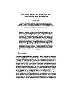
Fig. 1 shows the crystal lattice of a face cubic center (fcc) unit cell. The grey shaded triangle indicates one out of 4 possible planes, identified by its normal vector n, where gliding is most likely to occur, i.e. where the energy necessary to break loose the atomic bonds is lowest. Typically this is explained by comparing it with two densely packed plane arrays of spheres gliding on top of each other. With that picture in mind it becomes imaginable that there will be three preferred directions t for each such plane which minimize the resistance to relative motion of the slip planes. A so called “slip system” is defined by the dyadic product of the slip plane normal n and one out of 3 possible slip directions t, represented by the Schmid tensor mi = 12 (ti ⊗ ni + ni ⊗ ti ). (1) Consequently, in fcc crystals there are 3 x 4=12 slip systems. Double contraction of the Schmid tensor with the local stress tensor yields the resolved shear stress. Crystallographic slip on the nanoscale resulting in plastic yielding on the macroscopic scale is triggered when the resolved shear stress τi corresponding to the i-th
2
slip system reaches a critical value τc : τi = σ : m i ≤ τc
(2)
This condition represents the yield criterion on the crystallographic level. Generally it will be satisfied for multiple slip systems simultaneously, so the overall slip direction is made up by the combined action of active slip systems. In analogy to macroscopic theories the crystal plasticity theory has to provide an evolution law for the rate of deformation ε˙p which again is essentially a linear combination of the slip rates γ˙ i of the active slip systems. Note that the linear combination mathematically requires transforming the local slip rates into the global coordinate system again using the Schmid tensors in order to determine the overall rate of deformation: ε˙p =
X i
mi γ˙ i
(3)
The amount of slip in each direction in turn depends on the critical shear stress which again evolves due to hardening mechanisms that are commonly described by an interaction matrix hij , which also accounts for cross hardening effects of two active slip systems. Varying the entries into this matrix on the one hand allows to preclude certain non-physical combinations of slip systems, on the other hand it enables to activate otherwise idle slip systems in the wake of other already active ones: X τ˙ic = hij |γ˙ j | (4) j
τic = τ0 +
X
hij |γj |
(5)
j
Crystal plasticity uses the same formalism as known from classical plasticity theory, i.e. a yield criterion, equ. (2), the flow rule, equ. (3) and a hardening law (5). Corresponding to the plastic multiplier in standard plasticity a set of 12 variables γi is introduced representing the slip rates of each single slip system. Once these are determined, the overall plastic strain increment can be worked out using equ. (3). The elastic strain rate is found given an additive composition of the total strain rate, see equ. (6). (6) ε˙p + ε˙e = ε˙ Finally, using Hooke’s law the stress can be updated. The following section deals with the algorithmic details of determining the active set of slip systems and solving for the unknown slip rates. σ˙ = C ε˙e , (7) where C is the 4th -order elasticity tensor. The following section deals with the algorithmic details of determining the active set of slip systems and solving for the unknown slip rates.
3
z
n
t x r
y
Figure 1: Lattice structure of a unit cell with a face cubic centered (fcc) lattice structure. The shaded triangle represents one of the slip planes with the normal n. The slip direction is indicated by t.
3
Mathematical formalism
For the algorithmic implementation it is wise to store tensorial quantities such as the stress or strain tensor as vectors with 6 components as this is commonly done in finite element codes for structural problems. Also, it is a good idea to work with 24 slip systems instead of only 12. Such a concept distinguishes the gliding on a given slip plane in a given direction from gliding on exactly the same plane but in the opposite direction, thus treating it as two separate cases with only positive slip rates instead of a single slip system with the possibility of having negative slip rates. At the first glance introducing twice as many variables seems counterproductive in view of algorithmic simplicity. However, it becomes understandable considering the advantage of not having to deal with sign functions being the derivative of the absolute value function in equ (5). This way additional non-linearities can be avoided and the problem can be reduced to solving a linear set of equations, provided that there is no further non-linearity in the hardening law. Ultimately, for the numerical evaluation the problem has to be expressed in terms of algebraic equations, which requires integration of the equs. (3) and (6). With the notation of tensors as vectors one obtains δε = δεel + δεpl = δεel +
24 X
δγi mi ,
(8)
i=1
Since the integration is carried out implicitly the yield condition (2) has to be
4
formulated at time t + δt (again using vector notation): (σ + δσ)T mi ≤ τic (t + δt)
(9)
where the right hand side, in turn, evolves according to equ. (5). τic = τ0 +
X
hij (γj + δγj ).
(10)
j
Note that the absolute value can be omitted if we use 24 equations instead of only 12, i.e. 1 ≤ i, j ≤ 24. Then an additional constraint has to be satisfied: δγi ≥ 0
(11)
Equality in equ. (11) holds only if now gliding occurs. On the other hand gliding requires equality in equ. (9). Inequality in both equ. (9) and equ. (11) is mutually exlusive, which is commonly expressed by means of the Kuhn-Tucker condition which has to be satisfied at any time: [(σ + δσ)T mi − τic (t + δt)]δγi = 0
(12)
From the numerical point of view it is always easier to handle equations rather than inequalities when it comes to solving the problems for the unknowns δγj and δσ. Unfortunately, the equ. (12) is non-linear adding another degree of complexity to the problem. It is advisable to further simplify the problem formulation by reducing the number of unknowns. To this end we insert Hooke’s law (7) into equ. (9) taking into account that in vector notation the 4th -order elasticity tensor C is written as a second order 6 x 6 matrix Λ. mTi Λ(εel + δεel ) ≤ τ0 +
X
hij (γj + δγj )
(13)
j
The increment of the elastic strain vector δεel can be substituted from equ. (8), so we finally arrive at mTi Λ(εel + δε −
24 X
mk δγk ) ≤ τ0 +
X
hij (γj + δγj )
(14)
j
k=1
which contains only the slip increments δγj as unknowns. Note that the total strain increment δε is known and provided by the externally given strain history. Note also that generally all quantities are known at time t. The Kuhn-Tucker conditions will be satisfied if
³
´
mT Λ(εel + δε) − τ0 − i
24 X
hij (γj − δγj ) − mTi Λ
24 X
mj δγj δγi = 0,
1 ≤ i ≤ 24
j=1
j=1
(15) Judging from the structure of equ. (15) it is evident that the solution will be non-unique. Standard computation software such as MatLab will find one set of
5
δγi strongly depending on the start-vector provided by the user. The question which one out of all feasible solution sets will eventually appear in reality cannot be answered by mathematical means only. The answer is found in the principle of maximum dissipation, one of the most fundamental physical laws which has initially been formulated by Onsager in his pioneering work from the year 1931 [4]. It essentially states that all irreversible processes (and in the limit therefore also reversible processes) proceed in such a way that the corresponding dissipation rate becomes a maximum. In the present case the dissipation rate can be formulated as P =
24 X
τ0 γ˙ i → max .
(16)
i=1
Given a number of feasible solutions of equ. (15) the one which maximizes P has to be selected. Unfortunately there is no straightforward way of working out the complete set of solution sets other than systematically trying different start-vectors. Since such a method can be extremely time-consuming it is not yet suitable for the further use as material routine in continuum-mechanical calculations.
4
Conclusions
The classical relationships for crystal plasticity have been formulated in such a way as to make them accessible to a numerical treatment. A yield surface concept is presented where each single slip system corresponds to a hyperplane in stress space. The mathematical framework leads to a non-linear set of equations with the slip rates as solution variables. The question which one out of all feasible solutions of these equations eventually appear in reality is decided by means of the principle of maximum dissipation. A full implementation of this concept into a material routine of a continuum mechanics software requires efficient search strategies.
References [1] Schmid, E. and Boas, W., Plasticity of crystals, Chapman and Hall, London (1935). [2] Hill, R., Generalized constitutive relations for incremental deformation of metal crystals. J. Mech. Phys. Solids 14 (1966) 95–102. [3] Rice, J.R., Inelastic constitutive relations for solids: an internal variables theory and its application to metal plasticity. J. Mech. Phys. Solids 19 (1971) 433–455. [4] Onsager, L., Reciprocal relations in irreversible processes, Phys. Rev. 37 (1931).
6