reliability, 2-terminal reliability, and k-terminal reliability. â¢. The g-terminal reliability is the probability that every node in the network is able to communicate with ...
International Journal of Computer Applications (0975 – 8887) 9th International ICST Conference on Heterogeneous Networking for Quality, Reliability, Security and Robustness (QShine-2013)
An Algorithm for Enumeration of Terminal and Multi Terminal Paths in a Reliability Graph of Communication Networks Mohd Ashraf Saifi
Rajesh Mishra
School of ICT Gautam Buddha Univesrsity Greater Noida , India
School of ICT Gautam Buddha Univesrsity Greater Noida , India
ABSTRACT
2. PRELIMINARY AND ASSUMPTION
The mathematical theory of reliability has grown out of the demand of modern technology and particularly out of the experience with complex systems. The main objective is to enhance the ability of such complex network systems. This work present an efficient algorithm, which is a novel approach to generate all the minimal paths of the general flow network based on the principle of backtracking. It is a general flow network because, the proposed approach can find the minimal paths for multiple sources and multiple sinks in the network. One can further evaluate the network reliability using any existing SDP (Sum of Disjoint Products) based approach.
The networks studied here are s-t networks with two special cases: in first case it has been assumed to one single source node called s and one target node called t. Another case referred to multiple source node called s1, s2, s3,…sn and multiple target nodes called t1, t2, t3,…tn. The success or failure of these networks depends on whether or not there is a connection between the source node and destination node. Meanwhile, as links or nodes are failure free, the networks can be classified into three categories: Networks with node failures only : the obtained minimal cut sets are node minimal cut sets, Networks with link failures only : the minimal cut sets are link minimal cut sets, Networks with both node and link failures: in this case both node and link failures are considered. In this paper, only we consider networks in the second category, where each link is represented by an unordered pair of end nodes. For an link , v and w are said to be adjacent to each other, and the link is said to be incident with v and w. A path between v0 and vn in G is a sequence of distinct links ,< v1 , v2>,...,, and n is the length of the path.
General Terms Enumeration , Backtracking Algorithm, Sum of Disjoint Product, Multi Terminal, Multi Source
Keywords Path Sets, Cutsets. Network Reliability, Backtracking,
1. INTRODUCTION In recent years, network reliability measures have been used in various real time systems such as computer communication networks, power transmission, water distribution systems. Network reliability plays important role in our modern society [1]. Many research has been realized to evaluate the network reliability, most of them use are applicable only for single source and single terminal network based algorithms in terms of minimal cutset (MC) or minimal pathset (MP). When network grows in size and complexity increases, they become more and more prone to failures. So, reliability analysis is essential. A computer communication network may have number of vertices and edges in which vertices represent the physical location of systems (transmitters or receivers) and edges represent the communication links between them. The network is dependent upon the vertices or edges, in sense that, if vertices or edges fail, then the network can be considered to be failed. In order to avoid failure in network, all the minimal paths or cuts are considered so that any of the paths can be used to reach from source to destination. The paper is mainly divided into five sections. Section 2 presents some preliminaries and assumptions required in the rest of the paper. Section 3 is devoted to the literature survey. The proposed algorithm is given in Section 4. Section 5 presents the algorithm with illustration, and finally, Section 6 concludes the paper.
A graph is connected if there is a path between each pair of nodes in a graph. Henceforth we assume that all graphs considered here are connected and contain neither multiple links nor self-loop (i.e., links of the form ). There are three important measures to assess the performance of systems represented by a probabilistic graph: g-terminal reliability, 2-terminal reliability, and k-terminal reliability.
The g-terminal reliability is the probability that every node in the network is able to communicate with each other. The 2-terminal reliability is the probability that a communication exists between a specified pair of nodes in network. The k-terminal reliability ensures that a specified set of nodes of the network are able to communicate with each other. The network satisfies the following assumptions: Each node is perfectly reliable. The graph is connected. Each link has two states: working or failed. The states of links are statistically independent.
8
International Journal of Computer Applications (0975 – 8887) 9th International ICST Conference on Heterogeneous Networking for Quality, Reliability, Security and Robustness (QShine-2013)
3. SURVEY ON PATH/CUT AND NETWORK RELIABILITY Mishra and Chaturvesdi [21] provide surveys of the various definitions of reliability. They identified two distinct classes of reliability measures: deterministic and probabilistic. The deterministic criteria make use of discrete measures to define the reliability of a network. Ever since the application of the graph theory for terminal reliability (TR) evaluation was suggested [2, 3] a large number of algorithms have been proposed in the literature. The survey of the literature indicates that whole range of the TR algorithms can be classified into two broad categories [5], viz.,
Those which do not use path sets or cut sets (NPOC) but apply reduction/decomposition or transformation or a combination of these approaches.
Those which use path sets or cut sets as the starting point (POC).
However, NPOC based algorithms tend to be less efficient and uneconomical as compared to the algorithms based on POC approach [5]. Yeh [6] proposes using UGFM (Universal Generating Function Method) to search all minimal paths. To access the performance of systems there are three important measures are: g-terminal, 2-terminal and k-terminal reliability. The probability when each and every node is able to communicate with each other in the network is said to be g-terminal reliability and discussed in [7,8,9,10]. The probability when a specified pair of nodes can communicate in a network with each other is said to be 2-terminal reliability and when a specified set of nodes can communicate with each other in the network is said to be k-terminal reliability. Evaluating the kterminal reliability of a telecommunication networks is discussed in [11]. Luo et al [12] evaluates the k-terminal reliability using SDP (Sum of Disjoint Products) and MVI (Multi Variable Inversion) techniques. The k-terminal reliability evaluation using an algorithm based on Decomposition Technique is proposed in [13], [14] and using factoring theorem approach is discussed in [15], [16]. A graph reduction algorithm for networks with imperfect nodes is proposed in [17]. Ng-Hierarchical Network Polynomial (NHNP) proposed by Tony et al [18] is an efficient algorithm to compute the k-terminal reliability. To enumerate the k-trees using SDP approach can be seen in [19]. The MVI-SDP based method was first proposed in [20]. SDP helps to generate mutually disjoint terms, which in turn has one-to-one relationship with the network reliability expression.
4. PROPOSED ALGORITHM AND APPROACH A network is represented by a graph G (n, l), where n and l are number of nodes and branches of network, respectively. A directed graph is a connected graph, in which every branch has an orientation, between the specified source and sink/terminal nodes. Source node has no branch incident to it and the sink node has no branch incident from the node. Such a graph can always be represented by a connection matrix or adjacency matrix. There exists one-to-one correspondence between the two. Moreover, each nonzero element in each row is the node that is adjacent to the node represented by the row. In fact this forms the basis of tracing all path sets from the source to the sink node of a given network.
Once the connection matrix of the graph is available, the search starts with the source node, looks for nonzero elements in the connection matrix in the row corresponding to this node, and appends each nonzero entry separately in a new vector, where number of new vectors would be equal to the number of nonzero elements found in the search. It follows the same procedure for the last element added in each of these vectors, by selecting the row of connection matrix corresponding to these most recent entries till the sink node is met and thus builds several path sets in an ordered manner. The highlights of the method presented here can be summarized as:
It can find minimal paths for a specified pair of nodes. Path sets are obtained in increasing order. Terminal Numbering Convention is used, where the numbering begins at source node and terminates at terminal node and it is desired to enumerate all the path sets
The algorithm step are as follows: Step 1: Mark the arcs in network from 1 to n, source nodes being S1, S2.....Sn and destination nodes being -1,-2,-3…-n. Step 2: Create a linked data structure L = {{(Arcs of source node 1),( Arcs of source node 2)….(Arcs of Source node N)},{(Outgoing arcs from arc 1),( Outgoing arcs from arc2),….. (Outgoing arcs from arcN)}} of the network with the first “n” node of the link representing the outgoing arcs from each source node S1 to Sn. The remaining nodes form a link with every arc being linked to its source arc. Step 3: In order to define the minimal paths in the network, traverse the linked data structure from the source arc (S1…Sn) and follow until the destination is reached. Step 4: Create a working set (R) for pointing to the current arcs being considered in order to find if the arc is one amongst the minimal path. Step 4a: Point to the first arc in the working set (Ri). Step 4b: Check if the arc being pointed to (p) is the destination arc. If yes, print the minimal path, pop elements from stack (S) which has been added during the current traversal, delete the current set of arcs from queue (W) and backtrack. Step 4c: If p is not the destination arc, traverse through the working set until the node pointed by p is reached. Step4d: The node being pointed is the current set of arcs (V1…Vn) being considered for minimal paths. Step 5: Find if the current set of arcs (V1 to Vn) has already been visited. Step 5a: Check if (V1 to Vn) is already present in the queue (W) which contains the visited set of arcs. Step5b: If yes, Cycle is detected. Print the cycle, add the set of arcs (V1 to Vn) to the cycle queue (C), delete the current set of arcs from queue (W) and backtrack. If not, move to step 6. Step 6: Push the current arc being considered (p) to Stack (S) and add the current set of arcs being considered (V1…..Vn) to the queue (W) and loop to step 4. Step 7: Loop through 4 to 6 for rest of the arcs in working set (Ri).
5. ILLUSTARATION Consider 9-nodes, 13-links network as shown in Figure 1 below. Note that we have numbered to the source node, and to the terminal node.
9
International Journal of Computer Applications (0975 – 8887) 9th International ICST Conference on Heterogeneous Networking for Quality, Reliability, Security and Robustness (QShine-2013) Step 5: Since v={9,10} has not been visited and w={(3,4),(5,6),(7,8)}, move to step 6.
1
Step 6: Add 7 to S and v to W. Currently, S={7,5,3,1} and W={(3,4),(5,6),(7,8),(9,10)}.
S2
S1 2 11
Step 4: Since all arcs are not yet visited in the current working set, point p to the arc in current working set (9,10). So, p=9. Since p doesn’t point to the destination node, traverse through R to the node pointed by p. v={-1}.
12
3 6
5
4
Step 5: Since v={-1} has not been w={(3,4),(5,6),(7,8),(9,10)}, move to step 6.
7 9
8
13 -2
Figure 1: Two source node and two terminal node network Step 1: Consider a network with two source (S1 and S2), two destination (-1 and -2) nodes and 13 arcs. Mark the arcs from 1 to 13. Step 2: The linked data structure for the example network is created as follows: {{(1,2),(11,12)},{(3,4),(5,6),(5,6),(7,8),(7,8),(9,10),(9,10),(1),(-1),(-2),(9,10),(13),(-2)}}. Here, the first two nodes represent the outgoing arcs from source nodes while the rest of the nodes link each source arc with its outgoing arc. Step 3: Select the first source node (S1) to find the minimal path to reach the destination. Step 4: Working set is the set of arcs being considered for the first set of source nodes. In this example, the working set for the first set of source nodes is R={{(1,2)},{(3,4),(5,6),(5,6),(7,8),(7,8),(9,10),(9,10),(-1),(1),(-2),(9,10),(13),(-2)}}. Point p to the first arc (p=1). Since p doesn’t point to the destination node, traverse through R to the node pointed by p i.e. v={3,4}. Step 5: Since v={3,4} has not been visited and w=NULL, move to step 6. Step 6: Add 1 to S and v to W. Currently, S={1} and W={(3,4)}. Step 4: Since all arcs are not yet visited in the current working set, point p to the arc in current working set (3,4). So, p=3. Since p doesn’t point to the destination node, traverse through R to the node pointed by p. v={5,6}. Step 5: Since v={5,6} has not been visited and w={(3,4)}, move to step 6. Step 6: Add 3 to S and v to W. Currently, S={3,1} and W={(5,6)(3,4)}. Step 4: Since all arcs are not yet visited in the current working set, point p to the arc in current working set (5,6). So, p=5. Since p doesn’t point to the destination node, traverse through R to the node pointed by p. v={7,8}. Step 5: Since v={7,8} has w={(3,4),(5,6)}, move to step 6.
not
been
visited
and
Step 6: Add 9 to S and v to W. Currently, S={9,7,5,3,1} and W={(3,4),(5,6),(7,8),(9,10),(-1)}.
10
-1
visited
and
Step 6: Add 5 to S and v to W. Currently, S={5,3,1} and W={(3,4),(5,6),(7,8)}.
Step 4: Since all arcs are not yet visited in the current working set, point p to the arc in current working set (-1). So, p=-1. Since p has now reached the destination, pop elements from stack and delete the nodes from W. So, Minimal Path is {1,3,5,7,9}. Backtrack to the node (9,10) to consider the other outgoing arcs from the arc 9. Step 4: Since arc 9 leads to destination, move pointer p to 10. So, p=10. Since p doesn’t point to the destination node, traverse through R to the node pointed by p. v={-2}. Step 5: Since v={-2} has not been w={(3,4),(5,6),(7,8),(9,10)}, move to step 6.
visited
and
Step 6: Add 10 to S and v to W. Currently, S={10,7,5,3,1} and W={(3,4),(5,6),(7,8),(9,10),(-2)}. Step 4: Since all arcs are not yet visited in the current working set, point p to the arc in current working set (-1). So, p=-1. Since p has now reached the destination, pop elements from stack and delete the nodes from W. So, Minimal Path is {1,3,5,7,10}. Backtrack to the node (7,8) to consider the other outgoing arcs from the arc 7. Loop through for the rest of arcs to get the minimal path for first source (S1) to be: {(1,3,5,7,9),(1,3,5,7,10),(1,3,5,8),(1,3,6,9),(1,3,6,10),(1,4,7,9), (1,4,7,10),(1,4,8),(2,5,7,9),(2,5,7,10), (2,5,8),(2,6,9),(2,6,10),(11,9),(11,10),(12,13)}. Step 3 and 4: Once the minimal paths for first source is found out, move towards the second source and create the working set. R={{(11,12)},{(3,4),(5,6),(5,6),(7,8),(7,8),(9,10),(9,10),(-1),(1),(-2),(9,10),(13),(-2)}}. Follow the steps from 4 to 7 for this working set to find the minimal paths for source (S2) to be: {(9, 11),(10, 11),(12, 13)}
6. RESULT & DISCUSSION The proposed algorithm has been implemented and tested using C language. The results of various bench marks networks[4] tested on analysis are shown Figure 2. The experimental results on enumerated multi source - multi sink pathsets for a given general case networks tested and analyzed in Table 1.
Step 4: Since all arcs are not yet visited in the current working set, point p to the arc in current working set (7,8). So, p=7. Since p doesn’t point to the destination node, traverse through R to the node pointed by p. v={9,10}.
10
International Journal of Computer Applications (0975 – 8887) 9th International ICST Conference on Heterogeneous Networking for Quality, Reliability, Security and Robustness (QShine-2013)
[1] 9N12L
[2] 5N8L
[3] 21N26L
[4] 7N11L
[5] 16N24L
[7] 12N15L
[9] 8N9L
[6] 9N13L
[8] 14N21L
[10] 14N18L
Figure 2: Case networks tested on analysis
11
International Journal of Computer Applications (0975 – 8887) 9th International ICST Conference on Heterogeneous Networking for Quality, Reliability, Security and Robustness (QShine-2013)
Table: 1 Results for Enumeration of All Multi Source – Multi Sink Pathsets Fig No.
Network
Source Node Number
Terminal Node Number
Total MPs
Number of Minimal Pathset
1
9N12L
1
-1
8
{5, 8, 4, 6, 1} {5, 11, 10, 9, 4, 6, 1}, {12, 10, 9, 4, 6, 1}, {5, 11, 7, 1}, {12, 7, 1}, {5, 8, 3, 2}, {5, 11, 10, 9, 3, 2}, {12, 10, 9, 3, 2}
2
5N8L
1
-1
5
{6, 5, 1}, {8, 1}, {3, 2}, {6, 7, 2}, {6, 4}
3
21N26L
1
-1
18
{20, 16, 12, 7, 3, 1},{20, 23, 21, 17, 13, 8, 3, 1},{26, 25, 24, 22, 19, 18, 13, 8, 3, 1},{20, 16, 12, 7, 14, 10, 9, 4, 1},{20, 23, 21, 17, 13, 8, 14, 10, 9, 4, 1}, {26, 25, 24, 22, 19, 18, 13, 8, 14, 10, 9, 4, 1}, {26, 25, 24, 22, 19, 15, 11, 9, 4, 1}, {20, 16, 12, 7, 3, 5, 2}, {20, 23, 21, 17, 13, 8, 3, 5, 2}, {26, 25, 24, 22, 19, 18, 13, 8, 3, 5, 2}, {20, 16, 12, 7, 14, 10, 9, 4, 5, 2}, {20, 23, 21, 17, 13, 8, 14, 10, 9, 4, 5, 2}, {26, 25, 24, 22, 19, 18, 13, 8, 14, 10, 9, 4, 5, 2}, {26, 25, 24, 22, 19, 15, 11, 9, 4, 5, 2}, {20, 16, 12, 7, 14, 10, 6, 2}, {20, 23, 21, 17, 13, 8, 14, 10, 6, 2}, {26, 25, 24, 22, 19, 18, 13, 8, 14, 10, 6, 2}, {26, 25, 24, 22, 19, 15, 11, 6, 2}
4
7N11L
1
-1
9
{9, 1}, {8, 6, 2}, {10, 11, 6, 2}, {10, 7, 2}, {8, 4, 3}, {10, 11, 4, 3}, {8, 6, 5, 3}, {10, 11, 6, 5, 3}, { 10, 7, 5, 3}
5
16N24L
1
-1
17
{23, 17, 12, 9, 6, 5, 4, 3, 2, 1}, {23, 18, 14, 9, 7, 6, 5, 4, 3, 2, 1}, {24, 20, 14, 9, 7, 6, 5, 4, 3, 2, 1}, {23, 18, 15, 13, 7, 6, 5, 4, 3, 2, 1}, {24, 20, 15, 13, 7, 6, 5, 4, 3, 2, 1}, {24, 21, 19, 13, 7, 6, 5, 4, 3, 2, 1}, {23, 17, 12, 8, 5, 4, 3, 2, 1}, {23, 18, 14, 8, 5, 4, 3, 2, 1}, {24, 20, 15, 13, 7, 6, 5, 4, 3, 2, 1}, {24, 21, 19, 13, 7, 6, 5, 4, 3, 2, 1}, {23, 17, 12, 8, 5, 4, 3, 2, 1}, {23, 18, 14, 8, 5, 4, 3, 2, 1}, {24, 20, 14, 8, 5, 4, 3, 2, 1}, {23, 17, 11, 4, 3, 2, 1}, {23, 17, 10, 2, 1}, {23, 16, 1}, {22}
6
9N13L
1,2
-1, -2
16
{9, 7, 5, 3, 1}, {10, 7, 5, 3, 1}, {8, 5, 3, 1}, {9, 6, 3, 1}, {10, 6, 3, 1}, {9, 4, 7, 1}, {10, 7, 4, 1}, {8, 4, 1}, {9, 7, 5, 2}, {10, 7, 5, 2}, {8, 5, 2}, {9, 6, 2}, {10, 6, 2}, {9, 11}, {10, 11}, {13, 12}
7
12N15L
1,2
-1, -2
9
{13, 7, 2}, {11, 6, 1}, {12, 7, 2}, {12, 7, 3},{13, 7, 3}, {12, 8, 4}, {13, 8, 4}, {14, 9, 4}, {15, 10, 5}
8
14N21L
1
-1
15
{16, 9, 4, 1}, {16, 20, 17, 12, 6, 10, 5, 1}, {21, 17, 12, 6, 10, 5, 1}, {16, 9, 19, 18, 12, 6, 10, 5, 1}, {14, 13, 7, 10, 5, 1}, {16, 9, 19, 15, 13, 7, 10, 5, 1}, {14, 8, 11, 5, 1}, {16, 9, 19, 15, 8, 11, 5, 1}, {16, 20, 17, 12, 6, 2}, {21, 17, 12, 6, 2}, {16, 9, 19, 18, 12, 6, 2}, {14, 8, 3}, {14, 13, 7, 2}, {16, 9, 19, 15, 8, 3}, {16, 9, 19, 15, 13, 7, 2}
9
8N9L
1, 2, 3
-1, -2, -3
7
{6, 1}, {6, 2}, {7, 3}, {8, 3}, {7, 4}, {8, 4}, {9, 5}
10
14N18L
1, 2, 3, 4
-1, -2, -3
16
{ 8, 1}, {16, 9, 1}, {17, 10, 2}, {15, 18, 10, 2}, {17, 10, 3}, {15, 18, 10, 3}, {17, 11, 4}, {15, 18, 11, 4}, {16, 12, 4}, {17, 11, 5}, {15, 18, 11, 5}, {16, 12, 5}, {16, 13, 6}, {14, 6}, {16, 13, 7}, {14, 7}
*Here N represent the total number of node in a given network and L represent total links in the given network
7. CONCLUSION This paper proposes an algorithm to enumerate all multiterminal pathsets for evaluating reliability of multi-source and multi sink communication networks. This work proposes an algorithm to generate the entire minimal multi source – multi sink pathsets of the general flow network, which is a new approach and it is based on the principle of backtracking.
Further, one can evaluated the network reliability using existing SDP based approach proposed in Chaturvedi and Misra [1]. For the work presented in this paper, the algorithm has been translated and implemented in C language.
12
International Journal of Computer Applications (0975 – 8887) 9th International ICST Conference on Heterogeneous Networking for Quality, Reliability, Security and Robustness (QShine-2013)
8. REFERENCES [1] S.K. Chaturvedi and K.B.Misra 2002 “An efficient multivariable inversion algorithm for reliability evaluation of complex system using pathsets” International journal of reliability, quality, safety engineering, Vol. 9, No. 3 pp 237-259, [2] Misra K.B. and T.S.M. Rao 1982“Reliability analysis of redundant network using flow graph ” IEEE Transaction on Reliability, Vol. R-31, No.2, pp. 174-176, [3] Misra K.B. (Ed),1993 New Trends in System Relaibility Evaluation, Elsevier, Amsterdom. [4] Gebre B. A. and J.E. Ramirez-Marquez, 2007,Element Substitution Algorithm for Genral Two-terminal Network Reliability Analyses, IIE Transaction, Vol. 39, No. 3, pp. 265-275.
[11] Smail Adjabi and Kahina Bouchama, 2011 “k-terminal reliability Evaluation of a Telecommunications Network represented by Discrete and a Dynamic model” International Journal of Operation Research Vol. 8, No.3. [12] Tong Luo and K.S Trivedi, 1998 “An improved algorithm for Coherent System Reliability”, IEEE Transactions on Reliability, Vol.47, No.1. [13] A.Satyanarayan and M.K Chang, 1983 “Network Reliability and Factoring theorem,” Networks, vol.13. [14] R.K.Wood, 1986 “Factoring algorithm for computing kterminal reliability”, IEEE Transaction.Reliability, Vol. R-35. [15] L.B. Page and J.E.Perry, 1989 “A practical implementation of factoring theorem”, IEEE Transaction Reliability, vol.R-38, No.5.
[5] Misra K.B., Relaibility, 1992, Analysis and Predection: A Methodology Oriented Treatment, Elsevier, Amsterdom.
[16] L.B. Page and J.E. Perry, 1989, “Reliability analysis of directed networks using the factoring theorem”, IEEE Transaction. Reliability, Vol. R-38, No. 5.
[6] Wei-Chang Yeh, 2009, “A Simple Universal Generating Function Method to Search for all Minimal Paths in Network”, IEEE Transactions on Systems, Vol.39,No.6,November.
[17] O.R. Theologou and J.G.Carlier, 1991 “Factory and Reduction for networks with the imperfect nodes”, IEEE Transactions Reliability, Vol. 40, No.2.
[7] S.P.Jain and K.Gopal,1998 “An efficient algorithm for computing global reliability of a network”, IEEE Transaction Reliability, Vol.37,No.5,pp.488-492. [8] H.Feng and S.P.Chang, 1998 “A method of Reliability evaluation for computer communication networks”, IEEE International Symposium on Circuits and Systems,. [9] M.A.Aziz, M.A Sobana and M.A Samad, 1992, “Reduction of Computations in enumeration of terminal and multiterminal path set by method of indexing”, Microelectronics and Reliability, Vol.32, No.8. [10] .C.Monticone, 1993 “An implementation of buzacott algorithm for network global reliability”, IEEE Transaction Reliabiltiy, Vol.42, No.1.
[18] P.Ng Tony, 1991 “k-terminal Relaibility of hierarchical networks”, IEEE Transactions Reliability, Vol. 40, No. 2. [19] D. Rath and K.P. Somam, 1997 “A simple method for generating k-trees of a network,” Microelectronics and Reliability, Vol. 46, No. 2. [20] K.D. Heidtmann, 1989“Smaller sums of disjoint products by sub product inversion,” IEEE Transactions Reliability, vol. R-38, no.3, pp. 305-311. [21] R. Mishra and S.K. Chaturvedi, 2009 “A Cutsets-Based Unified Framework to Evaluate Network Reliability Measures” IEEE Transaction on Reliability, Vol. 58, No.4, pp. 658-666.
13