sequence is generated by a live capture (using a camera), ... and unacceptable for live video. ..... changes to two other people in another area of the backyard,.
An Algorithm for Lossless Smoothing of MPEG Video� Simon S. Lam, Simon Chow, and David K. Y. Yau Department of Computer Sciences The University of Texas at Austin Austin, Texas 78712
Abstract
International Standards Organization (ISO). The standard is known by the name of the working group, Moving Pictures Expert Group, that developed it [7]. MPEG has been developed for storing video (and associated audio) on digital storage media, which include CDROM, digital audio tapes, magnetic disks and writable optical disks, as well as delivering video through local area networks and other telecommunications channels. At rates of several Mbps, MPEG video is suitable for a large number of multimedia applications including video mail, video conferencing, electronic publishing, distance learning, and games.1 At this time, there are few alternative industry-wide standards. JPEG, another ISO standard and a precursor of MPEG, was designed for the compression of still images; it does not take into consideration the extensive frame to frame redundancy present in all video sequences. For teleconferencing and videotelephone applications, the CCITT H.261 standard speci es compression techniques at rates of p � 64 kilobits/second, where p ranges from 1 to about 30. Compared to H.261, the MPEG standard was designed for a higher range of rates and a much better visual quality. However, MPEG video is not intended to be broadcast television quality; other standards are being developed to address the compression of television broadcast signals at 10{45 Mbps.2 Full-motion video is a set of pictures displayed sequentially. In uncompressed form, each picture is a two dimensional array of pixels, each of which is represented by three values (24 bits) specifying both luminance and color information.3 From such uncompressed video data, an MPEG encoder produces a coded bit stream representing a sequence of encoded pictures (as well as some control information for the decoder). There are three types of encoded pictures: I (intracoded), P (predicted), and B (bidirectional). The sequence of encoded pictures is speci ed by two parameters: M , the distance between I or P pictures, and N , the dis-
Interframe compression techniques, such as those used in MPEG video, give rise to a coded bit stream where picture sizes di�er by a factor of 10 or more. As a result, bu�ering is needed to reduce (smooth) rate uctuations of encoder output from one picture to the next; without smoothing, the performance of networks that carry such video tra�c would be adversely a�ected. Various techniques have been suggested for controlling the output rate of a VBR encoder to alleviate network congestion or prevent bu�er over ow. Most of these techniques, however, are lossy, and should be used only as a last resort. In this paper, we design and specify an algorithm for lossless smoothing. The algorithm is characterized by three parameters: D (delay bound), K (number of pictures with known sizes), and H (lookahead interval). We present a theorem which guarantees that, if K � 1, the algorithm nds a solution that satis es the delay bound. (Although the algorithm and theorem were motivated by MPEG video, they are applicable to the smoothing of compressed video in general.) To study performance characteristics of the algorithm, we conducted a large number of experiments using statistics from four MPEG video sequences.
1 Introduction
Recent developments in digital video technology have made possible the storage and communication of full-motion video as a type of computer data, which can be integrated with text, graphics, and other data types. As part of our research project on the design of transport and network protocols for multimedia applications, we have been studying the characteristics of compressed digital video encoded in accordance with MPEG, which is a recently published standard of the
� Research supported in part by National Science Foundation grant no. NCR-9004464, and in part by an unrestricted grant from Lockheed. In Proceedings of ACM SIGCOMM '94, London, August 1994. 0
1 The target rate is 1.5 Mbps for a relatively low spatial reso-
lution, e.g., 350 � 250 pixels. 2 The quality of MPEG video has been compared to that of VHS recording [1]. 3 We use the term picture as in [3]. In this paper and the literature, the terms frame, image, and picture are often used interchangeably.
1
tance between I pictures. Thus, if M is 3 and N is 9, then the sequence of encoded pictures is I B B P B B P B B I B B P B B ::: where the pattern IBBPBBPBB repeats inde nitely. If M is 1 and N is 5, then the sequence is I P P P P I P P P P I P P P ::: where the pattern IPPPP repeats inde nitely. An interframe coding technique called motion compensation is used such that \pieces" of a P picture are obtained from the preceding I or P picture in the sequence, and pieces of a B picture are obtained from the preceding I or P picture and the subsequent I or P picture in the sequence. An I picture is intracoded; that is, it is encoded, and decoded, without using information from another picture. In general, an I picture is much larger than a P picture (in number of bits), which is much larger than a B picture. For typical natural scenes, the size of an I picture is larger than the size of a B picture by an order of magnitude. An MPEG encoder that compresses a video signal at a constant picture rate (e.g., 30 pictures/s) outputs a coded bit stream with a highly variable instantaneous bit rate. Such a coded bit stream is called variable bit rate (VBR) video. Packet-switching networks|such as ATM networks where transmission capacity is allocated on demand by statistical multiplexing|can in principle carry VBR video tra�c without a signi cant loss in bandwidth utilization. However, it is obvious, and has been demonstrated [10, 11], that the statistical multiplexing gain of nite-bu�er packet switches can improve substantially by reducing the variance of input tra�c rates.4 This is one of the objectives of the lossless smoothing algorithm to be presented in this paper. Changes in the output rate of an MPEG encoder should be viewed on three di�erent time scales: (1) from the encoding of one block to the next within a picture, (2) from one picture to the next within the video sequence being encoded, and (3) from one scene to the next within the video sequence. We will ignore rate uctuations during the encoding of a picture, since these uctuations can be smoothed out with a small amount of bu�ering at the encoder. The rate uctuations from one picture to the next are the most troublesome. Consider an I picture, which is 200,000 bits long, followed by a B picture, which is 20,000 bits long. (These are realistic numbers from some of the video sequences we have encoded at a spatial resolution of 640 � 480 pixels; see Figure 3 in Section 5.) Suppose the video application speci es a picture rate of 30 pictures/second. Transmitting the I picture in 1/30 second over a network would require a transmission capacity of 6 Mbps to be allocated. Then during the next 1/30 second, the transmission capacity required for the B picture drops precipitously to 0.6 Mbps. These very large uctuations are a consequence of the use of interframe coding techniques in MPEG. The encoder output rate also changes, on the average, as the scene in the video sequence being encoded changes. Pictures of more complex scenes require more bits to encode. Pictures also require more bits to encode when there is a lot 4 For a speci ed bound on loss probability.
of motion in a scene (P and B pictures in particular). We observed that the (smoothed) output rates from one scene to the next di�er by about a factor of 3 in the worst case, and thus are not as troublesome as rate uctuations between I and B pictures. The output rate of an MPEG encoder depends upon the spatial resolution of pictures (number of pixels) and the temporal resolution (picture rate), which are parameters typically speci ed by a multimedia application. The picture rate, as well as some other MPEG encoder parameters, can be adaptively controlled to modify the encoder output rate (see Section 3). Some researchers have described adaptive techniques for controlling the output rate of VBR encoders [2, 4, 9]. Since these VBR encoders are considered input sources of packet-switching networks, the techniques are sometimes referred to as source rate control or congestion control techniques. Most of these techniques are lossy. In this paper, we present an algorithm for smoothing picture-to-picture rate uctuations in a video sequence. The algorithm can be implemented in transport protocols for compressed video in general. The algorithm's performance, however, is improved by a lookahead strategy that makes use of the repeating pattern of I, P, and B pictures in an MPEG video sequence. The objective of the algorithm is to transmit each picture in the same pattern at approximately the same rate, while ensuring that the bu�ering delay introduced by the algorithm is bounded by D for every picture; the delay bound D is a parameter which is to be speci ed by the multimedia application. The algorithm is lossless because smoothing is accomplished by bu�ering, not by discarding some information. We believe that an algorithm such as ours should always be used in transmitting MPEG video over a network, while lossy techniques for rate control should be used only as a last resort to alleviate congestion. Solution to the problem of lossless smoothing is relatively straightforward if picture sizes are known a priori for all pictures in the video sequence.5 Our main contributions to be presented in this paper are: (1) the design of an algorithm with no knowledge of the sizes of pictures that have not yet been encoded, and (2) an experimental demonstration, using a set of MPEG video sequences, that our algorithm is e�ective|namely, the delay bound is satis ed for individual pictures and uctuations in the encoder output rate are reduced to minimum levels (i.e., to those uctuations caused by motion and scene changes in the video sequence). The balance of this paper is organized as follows. In Section 2, we provide an introduction to MPEG video|in particular, the structure of an MPEG video bit stream|from the perspective of designers of transport and network protocols. In Section 3, we describe techniques for adaptively controlling the output rate of an MPEG encoder, and explain why lossless smoothing should be used, and lossy techniques only as a last resort. In Section 4, the theoretical basis for algorithm design is stated in a theorem and a corollary. The algorithm is then designed and speci ed. In Section 5, we rst describe the MPEG video sequences used in our experiments. Experimental results are shown to illustrate the performance and demonstrate the e�ectiveness of our algorithm. Section 6 has some concluding remarks. 5 One such solution is given by Ott et al. [8].
2 MPEG Video
We describe in this section the structure of an MPEG video bit stream from the perspective of designers of transport and network protocols. For a conventional treatment, see Le Gall [3]; for details, consult the ISO standard [7]. Our observations of the e�ects of errors, introduced by manually changing some bits in the coded bit stream, can be found in an extended version of this paper [6]. Full-motion video is a set of pictures displayed sequentially. Each picture is represented as a two dimensional array of pixels, each of which is speci ed by a set of three values giving the red, green, and blue levels of the pixel. This is called the RGB representation. In MPEG encoding, each RGB triplet is rst transformed into a YCrCb triplet, where the Y value indicates luminance level and the Cr and Cb values represent chrominance (color information). As an illustration, a picture with a spatial resolution of 640 � 480 pixels and 24 bits per pixel requires about 921 kilobytes to represent when uncompressed. For a video sequence to be displayed at a picture rate of 30 pictures/s, the transmission capacity required is about 221 Mbps. For compression, MPEG uses intraframe techniques that exploit the spatial redundancy within a picture, as well as interframe techniques that exploit the temporal redundancy present in a video sequence. These are brie y described below. The structure of an MPEG video bit stream can be speci ed as follows in BNF notation: ::= f [ ] g
::= f g ::= f g ::= f g where the curly brackets f g delimit an expression that is repeated zero or more times. The sequence header contains control information (e.g., spatial resolution, picture rate) needed to decode the MPEG video bit stream. Pictures in an MPEG video sequence are organized into groups to facilitate random access; in particular, a time code speci ed in hours, minutes, and seconds is included in each group header. Repeating the sequence header at the beginning of every group of pictures makes it possible to begin decoding at intermediate points in the video sequence (facilitating random access). However, only the very rst sequence header is required; the others are optional. The header of a picture contains control information about the picture (e.g., picture type, temporal reference). The header of a slice contains control information about the
slice (e.g., position in picture, quantizer scale). Each header (sequence, group, picture, or slice) begins with a 32-bit start code that is unique in the coded bit stream|speci cally, the start codes are made unique by zero bit and zero byte stu�ing. Each macroblock in a slice represents an area of 16 � 16 pixels in a picture. For example, consider a picture of 640 � 480 pixels. There are 40 � 30 macroblocks in the picture. The macroblocks are placed in the coded bit stream sequentially in raster-scan order (left to right, top to bottom). It is natural to specify each row of macroblocks in the picture to be a slice. The picture, for the above example, would then be represented by a sequence of 30 slices, one for each row. However, the MPEG standard does not require that a slice contain exactly a row of macroblocks. By de nition, a slice contains a series of one or more macroblocks; the minimum is one macroblock, and the maximum can be all the macroblocks in the picture. Also slices in the same picture can have di�erent numbers of macroblocks. Each macroblock begins with a header containing information on the macroblock address, macroblock type, and an optional quantizer scale.6 However, the beginning of a macroblock is not marked by a unique start code, and thus cannot be identi ed in a coded bit stream. Furthermore, macroblocks are of variable length. Hence, a slice is the smallest unit available to a decoder for resynchronization. In particular, whenever errors are detected, the decoder can skip ahead to the next slice start code|or picture start code| and resume decoding from there. One or more slices would be missing from the picture being decoded. Macroblocks are the basic units for applying interframe coding techniques to reduce temporal redundancy. In an I picture, every macroblock is intracoded. In a P or B picture, a macroblock may be intracoded, or predicted using various interframe motion compensation techniques. Before describing motion compensation, we rst consider intracoded macroblocks and brie y describe the techniques for reducing spatial redundancy. To encode the luminance levels of the 16 � 16 pixels in a macroblock, the pixels are subdivided into four blocks of 8 � 8 pixels each. MPEG makes use of the fact that the human eye is less sensitive to chrominance than luminance. Therefore, the Cr and Cb planes are subsampled, i.e., for each macroblock, only 8 � 8 Cr (Cb) values are sampled, resulting in only one Cr block and one Cb block. Thus following the header of each intracoded macroblock, there are six blocks, each of which is coded as follows. Applying the discrete cosine transform (DCT) to the 64 values of a block produces 64 coe�cients that have a frequency domain interpretation. These coe�cients are quantized, with low-frequency coe�cients (of basis functions representing large spatial extent) quantized more nely than high-frequency coe�cients (of basis functions representing small detail). Signi cant compression is obtained when many coe�cients (typically the higher frequency ones) become zero after quantization. The above technique makes use of two facts: (1) the human eye is relatively insensi6 If speci ed, this would override the quantizer scale in the slice
header.
tive to high-frequency information, and (2) high-frequency coe�cients are generally small. Following quantization, the coe�cients are then run length coded to remove zeros, and then entropy coded (actually a combination of variable-length and xed length codes are used). Although both run length and entropy coding are lossless techniques, quantization is lossy (some image information is discarded).7 A macroblock in a P picture is predicted from the reference picture (i.e., the preceding I or P picture in the video sequence) as follows. Various algorithms may be used to search the reference picture for a 16 by 16 pixel area that closely matches this macroblock. (The algorithm is implementation dependent and not speci ed by the MPEG standard.) If prediction is used, two pieces of information are encoded: (1) a motion vector specifying the x and y translation to the matching area in the reference picture, and (2) an error term, specifying di�erences between the macroblock and the matching area. The motion vector is entropy coded, while both DCT and entropy coding are applied to the error term. Clearly, prediction is not used if it would take as many bits to code these two pieces of information as the macroblock's pixels; in this case, the macroblock can be intracoded as described above. Each B picture has two reference pictures, one in the past and one in the future. A macroblock in a B picture may be obtained from a matching area in the past reference picture (forward prediction), a matching area in the future reference picture (backward prediction), or an average of two matching areas, one in each of the two reference pictures (interpolation). For such predicted and interpolated macroblocks, motion vectors and error terms are encoded. But if necessary, a macroblock within a B picture can be intracoded. Since a B picture depends on a reference picture in the future, it cannot be encoded until the reference picture in the video sequence has been captured and digitized. To do so, an encoder must introduce a delay equal to the time to capture and digitize M pictures (less than or equal to M� , where 1=� is the picture rate of the encoder). Similarly, a decoder cannot decode a B picture until its reference picture in the future has been received. Thus, the order in which pictures are transmitted should be di�erent from the order in which a video sequence is displayed. Speci cally, the reference picture following a group of B pictures in a video sequence should be transmitted ahead of the group. For example, if the video sequence is I B B P B B P B B I B B P ::: Then the transmission sequence is I P B B P B B I B B P B B ::: .
3 Rate Control
In the networking literature, studies on peak rate control of VBR video are concerned with alleviating network congestion. In Section 3.1, we rst review techniques that can be 7 The techniques are essentially the same as those of JPEG.
Unlike MPEG, only intracoded pictures are speci ed by JPEG.
used for rate control, all of which are lossy. The smoothing problem of interest in this paper has a di�erent objective, and is unique to VBR video encoded using interframe techniques, such as MPEG video, which has di�erent types of pictures with a wide range of sizes. It has been demonstrated [10, 11] that the statistical multiplexing gain of a nite-bu�er packet switch (such as an ATM switch) can be increased by reducing the variance of its input tra�c.8 For the speci c objective of reducing picture-to-picture rate uctuations that are a consequence of interframe coding, lossless smoothing is a more appropriate solution than the lossy techniques. The problem of smoothing is introduced in Section 3.2. Design and speci cation of our smoothing algorithm are presented in Section 4.
3.1 Lossy techniques
An MPEG encoder can control its output rate by setting the quantizer scale in the slice header, and also setting the optional quantizer scale in the header of each macroblock within a slice. A coarser setting would result in a lower bit rate at the expense of poorer visual quality. Additionally, the encoder can also lower its output rate by discarding some of the high-frequency DCT coe�cients (under the assumption that the human eye is relatively insensitive to such high-frequency information). These rate control techniques are described in the MPEG standard as methods for ensuring that the input bu�er of the \model decoder" neither over ows nor under ows. As techniques to reduce the output rate of an encoder, both are lossy in that some information is discarded, and may result in visible artifacts in the decoded video. Each technique has been suggested as the basis of congestion control schemes for packet networks that carry VBR video tra�c. Speci cally, the encoder would control its output rate in response to feedback information from an entry point to a packet network or a point of congestion in the packet network [2, 4, 9]. These lossy techniques for rate control are inappropriate for reducing uctuations in the bit rate for transmitting I, B, and P pictures in MPEG video for the following reason. I pictures in MPEG video are about an order of magnitude larger than B pictures (see Figure 3 in Section 5).9 We experimented with changing the quantizer scale of an I picture from 4 to 30. The size of the picture is reduced from 282,976 bits to 75,960 bits. But the picture at the coarser quantizer scale (30) is grainy, fuzzy, and has visible blocking e�ects. Our observations are in agreement with the following statement from [3]: \Intracoded blocks contain energy in all frequencies and are very likely to produce `blocking effects' if too coarsely quantized; on the other hand, prediction error-type blocks contain predominantly high frequencies and can be subjected to much coarser quantization." 8 For a speci ed bound on loss probability. 9 This observation is consistent with the suggestion in [7] that,
for typical natural scenes, P pictures be allocated 2{5 times as many bits as B pictures, and I pictures be allocated up to 3 times as many bits as P pictures.
According to the above statement, I pictures should be quantized less coarsely than P and B pictures, not the other way around. Another lossy technique that has been suggested for network congestion control is to reduce the picture rate by dropping some B pictures from the video sequence being transmitted [2]. Although dropping B pictures would reduce the average rate of the video sequence, it does not address the problem of picture-to-picture rate uctuations of interest here. In summary, both spatial and temporal redundancy are greatly reduced in the coded bit stream of MPEG video. Any lossy technique to reduce the peak rate of the bit stream would degrade the visual quality of I pictures, the largest pictures by far in the video sequence. They are also the most important, since pieces of B and P pictures are obtained from the I pictures.
3.2 Lossless smoothing
Consider an MPEG video sequence with picture sizes, S1 ; S2 ; S3 ; : : : . The size sequence has large uctuations because I pictures are much larger than B pictures. However, in the video sequence (also the size sequence), there is a pattern of N picture types which repeats inde nitely. The objective of smoothing is to eliminate rate uctuations that are a consequence of interframe coding in MPEG. One way to accomplish this is to bu�er pictures (at the sending side of a transport protocol) so that each picture within the same pattern can be transmitted at the same rate. To illustrate, consider a video sequence with M = 3 and N = 9. The repeating pattern is IBBPBBPBB. Let Si ; Si+1 ; : : : ; Si+8 be the picture sizes of a particular pattern in the sequence. Let � denote the picture period (that is, the picture rate is 1=� ). Thus the objective of smoothing is to send each picture in this pattern at the following rate Si + Si+1 + : : : + Si+8 9� That is, the large I picture is transmitted at a smaller rate while the small B pictures are transmitted at a higher rate. Note that this averaging of rates is carried out on a pattern by pattern basis to smooth out picture-to-picture rate uctuations. However, the rate of the coded bit stream still uctuates from pattern to pattern. Such uctuations, however, are inherent characteristics of the video sequence (scene complexity and amount of motion), which cannot be reduced without sacri cing visual quality or incurring unacceptably long delays. We will refer to the above method as ideal smoothing. The ideal method has two disadvantages. First, if the video sequence is generated by a live capture (using a camera), the size of each picture is not known until it has been captured, digitized, and encoded. With the ideal method, the pictures in the same pattern would have to be bu�ered until all have been encoded|and the rate calculated for the pattern|before the rst picture in the pattern can be transmitted. In this case, the bu�ering delay would be very large,
Host
Encoder
λ(t)
ri
To network
Figure 1: System model for rate smoothing. and unacceptable for live video. Second, the ideal method described above does not ensure that the bu�ering delay of each picture is less than D, an upper bound which can be speci ed. In the next section, we design an algorithm for smoothing MPEG video with the objective that the delay incurred by each picture in the video sequence is less than D, a parameter that can be speci ed.
4 Smoothing Algorithm
Consider a video sequence that is to be displayed at the rate of 1=� pictures per second. � is called the picture period. We assume that the encoding (decoding) time of any picture in the video sequence is less than or equal to � seconds. We use Si to denote the size of picture i, i = 1; 2; 3; : : : ; which is the number of bits representing picture i in the coded bit stream. Both the system model and the algorithm described in this section can be used for compressed video in general. (The model and analysis presented in this section are from [5].) The presence of a repeating pattern in an MPEG video sequence is used to estimate the sizes of pictures that have not been encoded; it is, however, not needed in the system model, nor in the algorithm.
4.1 System model
The model for rate smoothing is a FIFO queue (with some modi cations). Input to the queue is from the output of an encoder (see Figure 1). At time t, let �(t) denote the output rate of the encoder (same as input rate of the queue) in bits/s. We do not know �(t) as a time function. It su�ces to assume that the Si bits encoding picture i arrive to the queue during the time interval from (i ? 1)� to i� . The server of the queue represents a channel (physical or logical) which sends the bits of picture i to a network at the rate of ri bits/s. This rate is calculated for picture i by an algorithm (which is to be designed and speci ed) whenever the server can begin sending picture i. The algorithm has three parameters that can be speci ed: K required number of complete pictures bu�ered in queue before the server can begin sending the next picture (0 � K � N ); speci cally, the server can begin sending picture i only if pictures i through i + K ? 1 have arrived (each has been completely encoded) D maximum delay speci ed for every picture in video sequence (seconds)
H
lookahead interval, in number of pictures, used by algorithm Note that if K is speci ed to be N , the algorithm has knowledge of all picture sizes needed for ideal smoothing.10 The delay of a picture is de ned to be the time of arrival of its rst bit to the queue to the time of departure of its last bit from the queue. (The delay, so de ned, includes the picture's encoding delay, queueing delay, and sending delay.) Note that the delay bound D must be speci ed such that
D � (K + 1)�
(1)
in order for the bound to be satis able. The case of K = 0 means that the server can begin sending the bits of picture i bu�ered in the queue before the entire picture i has arrived. We allow K = 0 to be speci ed for the algorithm. However, using K = 0 in an actual system gives rise to two problems. First, bu�er under ow is possible unless the encoder is su�ciently fast. Second, the algorithm can ensure that picture delays are bounded by D only if K � 1 (actually, if and only if K � 1; see Theorem 1 in Section 4.2). The parameter, H , is for improving algorithm performance by looking ahead (even though only the pattern is known, but not necessarily picture sizes). Its meaning will become clear in Section 4.3. We next de ne the following notation: ti time when server can begin sending picture i di departure time of picture i (the server has just sent the last bit of picture i) Additionally, at time ti , the algorithm calculates the rate ri . To simplify notation, and without loss of generality, the calculation is assumed to take zero time. The following equation de nes the meaning of parameter K ,
ti = maxfdi?1 ; (i ? 1 + K )� g
(2) That is, the server can begin sending picture i only after picture i ? 1 has departed and pictures i; i +1; : : : ; i ? 1+ K , have arrived (i.e., encoded and picture sizes are known). The departure time of picture i is di = ti + (Si =ri ) (3) and the delay of picture i is delay i = di ? (i ? 1)� (4) Note that in an actual system, the encoding of picture i ? 1+ K may be complete at time y, such that (i ? 2+ K )� < y � (i ? 1 + K )� . Also the rst bit of picture i may arrive at time x, such that (i ? 1)� < x < i� . We use (i ? 1 + K )� in Eq. (2) and (i ? 1)� in Eq. (4) because �(t) is unknown. If either x or y were known and used instead, the delay of each picture may be smaller than the value calculated using (2){(4), but the di�erence would be negligible. 10 Some modi cation is needed to ensure that the delay of each
picture is less than D.
4.2 Upper and lower bounds on rate
We present an upper bound and a lower bound on the rate ri that can be selected by an algorithm for sending picture i at time ti , for all i. The lower bounds are used to ensure that the delay of each picture is less than or equal to D. We say that the algorithm satis es delay bound D if for i = 1; 2; : : : delay i � D The upper bounds on rates are used to ensure that the server works continuously. If rates are too large, then the server may send bits faster than the encoder can produce them, forcing the server to idle, i.e., the server cannot send the next picture because the queue does not have K complete pictures.11 We say that the algorithm satis es continuous service if for i = 1; 2; : : : ti+1 = di It might be argued that the delay bound is a more important property than the continuous service property. However, there is no need to choose, because Theorem 1 below shows that both properties can be satis ed. An assumption of Theorem 1 is that Si is known at time ti , which can be guaranteed by specifying K to be greater than or equal to 1. If Si is not known at time ti (i.e., K is speci ed to be 0), it is easy to construct examples such that the delay bound cannot be satis ed.
Theorem 1 If Si is known at ti , and ri is selected for i = 1; 2; : : : ; n such that conditions (5) and (6) hold,
ri � D + (i ?Si1)� ? t
i
(5)
ri � (i + KS)i� ? t if ti < (i + K )� (6) i then for i = 1; 2; : : : ; n, (7), (8) and (9) in the following hold: delay i � D (7) ti+1 < i� + D (8) ti+1 = di (9) Theorem 1 is proved by induction on n. A proof can be
found in [5, 6]. We use riL and riU to denote the lower bound in (5) and the upper bound in (6), respectively. For these upper and lower bounds, we say that a bound is well de ned if its denominator is positive; see (5) and (6). In Theorem 1, (8) guarantees that the lower bounds are all well de ned. As for the upper bounds, many in (6) may not be well de ned. These are de ned as follows: riU = 1 if ti � (i + K )�: Because of (1), the following corollary is immediate.
Corollary 1 For all i = 1; 2; : : : ; n, riL � riU
(10)
Corollary 1 implies that both the delay bound and the continuous service property can be satis ed. 11 For K = 0, bu�er under ow may occur.
4.3 Lookahead to improve algorithm performance
Theorem 1 requires that the rate for picture i be chosen from the interval [riL ; riU ], which may be large if D > (K + 1)� . This exibility can be exploited to reduce the number of rate changes over time. Suppose the sizes of pictures i, i +1, i +2, : : : are known. The algorithm can be designed to nd a rate for sending pictures i through i + h, for as large a value of h as possible. In our system model, however, the size of picture j; j > i + K ? 1, may not be known at time ti . Speci cally, for K = 1, it is likely that Sj , j > i, has to be estimated. Fortunately, Theorem 1 requires only Si to be known at ti . Sizes of pictures arriving in the future may be estimated without a�ecting Theorem 1. In what follows, we derive a set of upper bounds and a set of lower bounds from Si ; Si+1 ; Si+2 ; : : : ; where Sj ; j > i + K ? 1, may be an estimate. There are many ways to estimate the size of a picture from past information. In the experiments described in Section 5, the size of picture j , if not known at ti , was estimated to be Sj?N . This is a simple estimate which uses the fact that pictures j ? N and j are of the same type (I, B or P) in MPEG video. They are about the same size unless there is a scene change in the picture sequence from j ? N to j . If all pictures in the future are sent at the rate ri , the (approximate) delay of picture i + h; h = 0; 1; 2; : : : ; is h X
ti + m=0
Si+m
ri
? (i ? 1 + h)�
(11)
Requiring the above to be � D, we have h X m=0
Si+m
ri � D + (i ? 1 + h)� ? t
i
(12)
where the lower bound on ri will be denoted by riL (h). The (approximate) departure time of picture i + h is h X
Si+m
di+h = ti + m=0r
i
The continuous service property requires that di+h � (i + h + K )� , which can be satis ed by requiring h X
Si+m
ri � (i +mh=0+ K )� ? t
i
if ti < (i + h + K )�
(13)
where the upper bound on ri will be denoted by riU (h) if ti < (i + h + K )� ; else, riU (h) is de ned to be 1. Note that riL (0) and riU (0) are equal to the lower bound riL and upper bound riU , respectively, given in Theorem 1. Also, only riL (h) and riU (h) for h = 0; 1; : : : ; K ? 1 are accurate bounds; the others, calculated using estimated picture sizes, are approximate.
A strategy to reduce the number of rate changes over time is to rst nd the largest integer h� such that max rL (h) � 0�min rU (h) (14) 0�h�h� i h�h� i
The rate ri for picture i is then selected such that for h = 0; 1; : : : ; h� riL (h) � ri � riU (h) Note that for K � 1, the selected rate satis es riL = riL (0) � ri � riU (0) = riU Therefore, the hypothesis of Theorem 1 holds and the delay bound D as well as the continuous service property are satis ed even though picture sizes (namely, Sj ; j > i) are estimated. To minimize delay, we would like to use K = 1 in the algorithm, in which case most picture sizes are estimated. For this reason, the smoothing algorithm in Section 4.4 is designed with a parameter H which can be speci ed. Instead of searching for the largest h� satisfying (14), the search is limited to a maximum value of H ? 1. For MPEG video, we conjecture that there is no advantage in having H greater the size of a pattern (N ) because picture sizes are estimated using past information. We conducted experiments to study this conjecture and found that it is supported by experimental data; see Section 5.
4.4 Algorithm design and speci cation
The smoothing algorithm is designed using (2){(4), (12){ (14), Theorem 1, and Corollary 1. A speci cation of the basic algorithm is given in Figure 2. The following are assumed to be global variables: pic size: array [index] of integer; seq end: boolean; tau: real; The value of pic size[i] is Si in the system model, the value of tau is the picture period, and seq end, initially false, is set to true when the algorithm reaches the last picture of a video sequence. There are three functions in the speci cation: max, min, and size. In particular, size(j;t) returns, at time t, either the actual size of picture j or an estimated size (in number of bits). For the experimental results presented in Section 5, we used the following simple estimation based upon the fact that a known pattern of N picture types repeats inde nitely in MPEG video:
if (t � j � tau) then return pic size[j ] else return pic size[j ? N ] For the initial part of a video sequence, where pic size[j ? N ] is not de ned, each I picture is estimated to be 200,000
bits, each P picture 100,000 bits, and each B picture 20,000 bits. These estimates are far from being accurate for some video sequences. But by Theorem 1, they do not need to be accurate. An MPEG encoder may change the values of M and N adaptively as the scene in a video sequence changes. Note
procedure smooth(H , K : integer; D: real); var i, h, sum: integer;
depart, time, rate, delay, lower, upper, lower old, upper old: real; begin i := 0; depart := 0:0; seq end := false; repeat i := i + 1; time := max(depart, (i ? 1 + K ) � tau); ftime to begin sending picture ig h:=0; sum:=0; lower:=0.0; upper:=1;
repeat
sum := sum + size(i + h, time); lower old := lower; upper old := upper; lower := sum/(D + (i ? 1 + h) � tau? time); if (time � (K + i + h) � tau) then upper:=1 else upper := sum/((K + i + h) � tau? time); lower := max(lower, lower old); upper := min(upper, upper old); h := h + 1; until (lower > upper) or (h � H ); if (lower > upper) then if (lower > lower old) then rate:=upper fupper=upper oldg else rate := lower flower = lower old, upper < upper oldg else fh = H g if (i = 1) then rate:=(lower+upper)/2; frate for rst pictureg else fpossible modi cation hereg if (rate>upper) then rate:=upper else if (rate < lower) then rate := lower; notify(i, rate); fnotify transmitter the rate for picture ig depart := time + pic size[i]/ rate; fdeparture time of picture ig delay := depart ?(i ? 1) � tau fdelay of picture ig until seq end end; fsmoothg
Figure 2: Speci cation of basic algorithm. that the basic algorithm does not depend on M , and it uses N only in picture size estimation. Lastly, we use notify(j;r) to denote a communication primitive which noti es a transmitter that picture j is to be sent at rate r. Note that the inner repeat loop calculates the bounds in (14). The loop has two exit conditions. The exit condition, (lower > upper), corresponds to h� in (14) being less than H ? 1; when this happens (called early exit), it can be proved that one of these two conditions holds: � lower > lower old and upper = upper old � lower = lower old and upper < upper old The selection of ri in each case is designed to minimize the number of rate changes over time. The second exit condition corresponds to h� in (14) being larger than or equal to H ? 1 (called normal exit); in the
algorithm, the search for h� stops at h = H ? 1 because the lookahead interval is limited to H pictures. Upon normal exit, ri is selected to be the same as ri?1 , i.e., no rate change unless the current value of rate is larger than upper or smaller than lower. This selection strategy is designed to minimize the number of rate changes. We also investigated a variation of the basic algorithm such that the moving average calculated using rate := sum=(N � tau) (15) is selected for ri (unless the moving average is larger than upper or smaller than lower). To modify the algorithm, the assignment statement in (15) replaces the comment \fpossible modi cation hereg" in procedure smooth. The modi ed algorithm produces numerous small rate changes over time, but its rate r(t), as a function of time, tracks the rate function of ideal smoothing more closely than the basic algorithm. In particular, the area di�erence (a performance measure de ned in Section 5) is smaller.
5 Experiments
To show that the smoothing algorithm is e�ective and satis es the correctness properties given in Theorem 1, we performed a large number of experiments using four MPEG video sequences. Some of our experimental results are shown in Figures 4{8 and discussed below. For all experiments, the picture rate is 30 pictures/s.
5.1 MPEG video sequences
Driving1 (N = 9, M = 3) and Driving2 (N = 6, M = 2)
This video was chosen because we thought that it would be a di�cult one to smooth. There are two scene changes in the video. Initially, the scene is that of a car moving very fast in the countryside. The scene then changes to a close-up of the driver, and then changes back to the moving car. This video is encoded twice, using di�erent coding patterns, to produce two MPEG video sequences. Note, from Figure 3, that the scene changes give rise to abrupt changes in picture sizes. In particular, P and B pictures in the driving scenes are much larger than P and B pictures in the close-up scene. The pictures were encoded with a spatial resolution of 640 � 480 pixels. Tennis (N = 9, M = 3) This video shows a tennis instructor initially sitting down and lecturing. He then gets up to move away. There is no scene change in the video. But as the instructor gets up, his motion gives rise to increasingly large P and B pictures. These changes in picture sizes are gradual. However, there are two isolated instances of large P pictures in the rst half of the sequence. The pictures were encoded with a spatial resolution of 640 �480 pixels. Backyard (N = 12, M = 3) There are also two changes of scene in this video. Initially, the scene is that of a person in a backyard. The scene
Coding pattern:IBBPBBPBB
Driving1
Coding pattern: IBBPBBPBB 350000 I P B
250000
I P B
300000
200000
250000
bits/picture
bits/picture
Tennis
150000
200000
150000
100000 100000 50000 50000
0
0 0
50
100
150 picture number
200
250
300
0
50
100
150 picture number
200
250
300
Figure 3: Two MPEG video sequences. changes to two other people in another area of the backyard, and then changes back to the rst person. The backgrounds of both scenes are complex with many details. While there are movements, the motion is not rapid. The pictures were encoded with a spatial resolution of 352 � 288 pixels. Due to space limitation, only Driving1 and Tennis are shown in Figure 3.
5.2 Performance of the basic algorithm
For the Driving1 sequence, Figure 4 shows bit rate as a function of time for K = 1, H = 9, and four values of the delay bound D. In each case, we compare the rate function from the basic algorithm, denoted by r(t), with the rate function from ideal smoothing, denoted by R(t). From Figure 4, we see that the \smoothness" of r(t) improves as the delay bound is relaxed. (We will de ne some quantitative measures of smoothness below.) For D = 0:1 second, r(t) does not look smooth at all, even though it is a lot smoother than the rate function �(t) of the MPEG encoder output. (If �(t) is not smoothed, the largest I picture would require over 7.5 Mbps to send in 1/30 second.) Note that the improvement in smoothness from D = 0:2 second to D = 0:3 second is not signi cant. Therefore, D = 0:2 second would be an excellent parameter value to use if a delay of up to 0.2 second (which includes encoding delay) is an acceptable price to pay for a smoothed output. Note that the smoothed rate function of the Driving1 sequence varies from about 1 Mbps to 3 Mbps. These variations are due to di�erences in the content and motion of scenes. These rates depend upon the spatial resolution (640 � 480) and quantizer scales (4 for I, 6 for P, and 15 for B) speci ed for encoding the sequence. For the Driving1 sequence, Figure 5 shows the delays of pictures for two comparisons. In the graph on the left, we compare these three cases: � D = 0:1 second, K = 1, H = 9, basic algorithm � D = 0:3 second, K = 1, H = 9, basic algorithm � ideal smoothing
As shown, the delays of pictures are bounded by 0.1 second and 0.3 second as speci ed for the basic algorithm. For ideal smoothing, picture delays are large, due to the requirement that pictures in the same pattern are bu�ered until all have arrived before the rst picture in the pattern can be transmitted. In the graph on the right of Figure 5, we compare these three cases � K = 1, H = 9, D = 0:1333 + (K + 1)=30 second, basic algorithm � K = 9, H = 9, D = 0:1333 + (K + 1)=30 second, basic algorithm � ideal smoothing For K = H = N = 9, the smoothing algorithm does not estimate picture sizes. In this case, the basic algorithm is very similar to ideal smoothing.12 A comparison of the delays for the two cases, K = 1 and K = 9, shows the desirability of using K = 1. The slack in the delay bound is chosen to be the same, 0.1333 second, so that the smoothness of r(t) is about the same in both cases (see discussion on Figure 8 below). No \delay bound violation" has been observed in any of our experiments where K � 1. This is not surprising, since the absence of delay bound violation is guaranteed by Theorem 1 if K � 1. For K = 0, however, we did observe some delay bound violations when the slack in the delay bound was deliberately made very small. Di�erent quantitative measures can be de ned to characterize the e�ectiveness of smoothing. We use four of them to study algorithm performance as each of the parameters, D, H , K , varies. The rst measure is de ned as follows: RT [r(t) ? R(t + (N ? K )� )]+ dt Area di�erence = 0 R T (16) 0 R(t + (N ? K )� ) dt where T denotes the time duration of the video sequence. Note that with ideal smoothing, picture 1 begins transmission (N ? K )� seconds later than if the basic algorithm were
12 They are not identical, because ideal smoothing as described
in Section 3.2 does not try to keep the delay of each picture less than a speci ed bound D.
4
4 Driving1 K=1, H=9
Ideal D=0.15
3.5
3.5
3
3
2.5
2.5 Rate (Mbps)
Rate (Mbps)
Ideal D=0.10
2
2
1.5
1.5
1
1
0.5
0.5
0
Driving1 K=1, H=9
0 0
2
4
6
8
10
0
2
4
Time (seconds)
4
8
10
8
10
4 Ideal D=0.20
Driving1 K=1, H=9
Ideal D=0.30
3.5
3.5
3
3
2.5
2.5 Rate (Mbps)
Rate (Mbps)
6 Time (seconds)
2
2
1.5
1.5
1
1
0.5
0.5
0
Driving1 K=1, H=9
0 0
2
4
6
8
10
Time (seconds)
0
2
4
6 Time (seconds)
Figure 4: Rate as a function of time for four delay bounds (Driving1 sequence, basic algorithm). used. Therefore the rate function from ideal smoothing is shifted by this much time in (16). Only the positive part of the di�erence between r(t) and R(t) is used in (16) because of the following: Z T
0
[r(t) ? R(t + (N ? K )� )] dt = 0
We use three other measures: � the number of times r(t) is changed by the algorithm over [0; T ] � the maximum value of r(t) over [0; T ] � the standard deviation (S.D.) of r(t) over [0; T ] Figure 6 shows the four quantitative measures as a function of delay bound D for the four MPEG video sequences. All four measures indicate that as the delay bound is increased (relaxed), the rate function r(t) becomes more smooth. The Backyard sequence appears to be the easiest to smooth. For the three MPEG video sequences encoded at a spatial resolution of 640 � 480 pixels, the maximum smoothed rate is about 3 Mbps. For the Backyard sequence encoded at a spatial resolution of 352 � 288 pixels, the maximum smoothed rate is about 1.5 Mbps, which is about the target rate of the MPEG standard. The maximum (smoothed) rate versus D curves in Figure 6 represent
a valuable design tradeo� made possible by lossless smoothing. Figure 7 shows the quantitative measures as a function of the lookahead interval, H , for the four MPEG video sequences. In Section 4.3, we conjectured that because most picture sizes are estimated using past information, there is no advantage in having H larger than the size of the repeating pattern (N ). Our experimental data support this conjecture. In Figure 7, the area di�erence, standard deviation of rate, and maximum rate do not show any noticeable improvement for values of H larger than N . In fact, the number of rate changes increases as H increases. K should be as small as possible to reduce picture delay. Theorem 1 requires K � 1. We conducted experiments to investigate whether there is any improvement in smoothness of r(t) from using K > 1. Figure 8 shows that there is a small improvement as K increases, but barely noticeable. Note that the delay bound is D = 0:1333+(K +1)=30, with a constant slack of 0.1333 for all cases. We conclude that K = 1 should be used.
6 Conclusions and Related Work As part of our research project on the design of transport and network protocols for multimedia applications, we studied
MPEG video. We found that interframe compression techniques, such as the ones speci ed by MPEG, give rise to a coded bit stream in which picture sizes di�er by a factor of 10 or more. As a result, some bu�ering is needed to smooth the picture-to-picture rate uctuations in the coded bit stream; otherwise, the very large uctuations would make it very di�cult to allocate a communication channel (based upon either packet switching or circuit switching) with appropriate quality-of-service guarantees. Some researchers have described techniques for controlling the output rate of VBR encoders [2, 4, 9]. Most of these techniques are lossy, and are inappropriate for smoothing picture-to-picture rate uctuations that are a consequence of interframe compression. For alleviating network congestion, the lossy techniques may be used in addition to lossless smoothing. However, they should be used only as a last resort, because both the spatial and temporal redundancy present in video are greatly reduced in MPEG bit streams. On the other hand, a lossless algorithm, such as the one presented in this paper, should always be used to smooth out rate uctuations from interframe compression. Our algorithm is designed to satisfy a delay bound, D, which is a parameter that can be speci ed. The algorithm is characterized by two other parameters, K , the number of pictures with known sizes, and, H , a lookahead interval for improving algorithm performance. We also presented a theorem which states that if K � 1, then our algorithm satis es both the delay bound D and a continuous service property. Although our system model and algorithm, as well as Theorem 1, were motivated by MPEG video, they are applicable to compressed video in general. We make use of the assumption that there is a known pattern of picture types which repeats inde nitely in the video sequence, to estimate picture sizes. Such size estimates are used in a lookahead strategy to improve algorithm performance. The problem of smoothing was analyzed by Ott et al. [8], where picture sizes in a video sequence are assumed to be known a priori. The parameter K is absent in their model, and there is no notion of a repeating pattern [8]. From a practical point of view, K is a crucial parameter for any smoothing algorithm. Furthermore, Theorem 1 shows that there is no need to assume all picture sizes to be known a priori. Instead, we use a known pattern and estimated picture sizes in our algorithm. We conducted a large number of experiments using statistics from four MPEG video sequences to study the performance of our algorithm. We found that it is e�ective in smoothing rate uctuations, and behaves as described by Theorem 1. Experimental data suggest that the following choice of parameters provides a smooth rate function: K = 1, H = N , and D = 0:2 second. The delay bound includes the encoding delay of each picture. A larger delay bound does not seem to provide any noticeable improvement in the smoothness of the resulting rate function. In the case that a multimedia application requires a smaller delay bound, the rate uctuations would be noticeably larger.
Acknowledgements
We thank Thomas Y. C. Woo for his technical comments and his help in the preparation of gures. We also thank the referees for their constructive comments.
References
[1] M. Anderson. VCR quality video at 1.5 Mbits/s. In National Communication Forum, October 1990. [2] L. Delgrossi, C. Halstrick, D. Hehmann, R. G. Herrtwich, O. Krone, J. Sandvoss, and C. Vogt. Media scaling for audiovisual communication with the Heidelberg transport system. In Proceedings of ACM Multimedia '93, pages 99{104, August 1993. [3] D. Le Gall. MPEG: A video compression standard for multimedia applications. CACM, 34(4):46{58, April 1991. [4] H. Kanakia, P. Mishra, and A. Reibman. An adaptive congestion control scheme for real-time packet video transport. In Proceedings of ACM SIGCOMM '93, pages 20{31, September 1993. [5] S. S. Lam. A model for lossless smoothing of compressed video, January 1994. Unpublished manuscript (presented at Experts on Networks Symposium, 60th birthday of Professor Leonard Kleinrock, UCLA, June 1994). [6] S. S. Lam, S. Chow, and D. K. Y. Yau. An algorithm for lossless smoothing of MPEG video. Technical Report TR-9404, Department of Computer Sciences, University of Texas at Austin, February 1994. [7] Coding of moving pictures and associated audio, November 1991. SC29/WG11 committee (MPEG) draft submitted to ISO-IEC/JTC1 SC29. [8] T. Ott, T. Lakshman, and A. Tabatabai. A scheme for smoothing delay-sensitive tra�c o�ered to ATM networks. In Proceedings of INFOCOM '92, pages 776{785, 1992. [9] P. Pancha and M. El Zarki. Bandwidth requirements of variable bit rate MPEG sources in ATM networks. In Proceedings of INFOCOM '93, pages 902{909, March 1993. [10] A. Reibman and A. Berger. On VBR video teleconferencing over ATM networks. In Proceedings of GLOBECOM '92, pages 314{319, 1993. [11] D. Reininger, D. Raychaudhuri, B. Melamed, B. Sengupta, and J. Hill. Statistical multiplexing of VBR MPEG compressed video on ATM networks. In Proceedings of INFOCOM '93, pages 919{925, March 1993.
0.6
0.6 Ideal D=0.10 D=0.30
Driving1 K=1, H=9
0.5
Delay of picture (seconds)
0.5
Delay of picture (seconds)
Ideal K=1 K=9
Driving1 D=0.1333 + (K+1)/30, H=9
0.4
0.3
0.2
0.1
0.4
0.3
0.2
0.1
0
0 50
100
150 picture number
200
250
50
100
150 picture number
200
250
Figure 5: Delays of pictures in Driving1 sequences (basic algorithm).
0.45
2.5 Driving 1 Driving 2 Tennis Backyard
K=1, H=N 0.4
Driving 1 Driving 2 Tennis Backyard
K=1, H=N
2
0.35
S.D. of rate (Mbps)
Area difference
0.3
0.25
0.2
1.5
1
0.15
0.1
0.5
0.05
0 0.05
0.1
0.15
0.2 D (seconds)
0.25
0.3
0 0.05
0.35
300
0.1
0.15
0.2 D (seconds)
0.25
0.3
0.35
9 Driving 1 Driving 2 Tennis Backyard
K=1, H=N 250
Driving 1 Driving 2 Tennis Backyard
K=1, H=N 8
7
No. of rate changes
Maximum rate (Mbps)
200
150
100
6
5
4
3
2 50 1
0 0.05
0.1
0.15
0.2 D (seconds)
0.25
0.3
0.35
0 0.05
0.1
0.15
0.2 D (seconds)
0.25
Figure 6: Performance of basic algorithm as a function of delay bound D.
0.3
0.35
0.4
S.D. of rate (Mbps)
0.3
Area difference
1.5
Driving 1 Driving 2 Tennis Backyard
D=0.2, K=1
0.2
Driving 1 Driving 2 Tennis Backyard
D=0.2, K=1
1
0.5
0.1
0
0 0
2
4
6
8
10
12
14
16
18
0
2
4
6
8
H
250
12
14
16
18
8 Driving 1 Driving 2 Tennis Backyard
D=0.2, K=1
Driving 1 Driving 2 Tennis Backyard
D=0.2, K=1
Maximum rate (Mbps)
200
No. of rate changes
10 H
150
100
6
4
2 50
0
0 0
2
4
6
8
10
12
14
16
18
0
2
4
6
H
8
10
12
14
16
18
H
Figure 7: Performance of basic algorithm as a function of parameter H .
0.4
S.D. of rate (Mbps)
0.3
Area difference
1.5
Driving 1 Driving 2 Tennis Backyard
D=0.1333 + (K+1)/30, H=N
0.2
Driving 1 Driving 2 Tennis Backyard
D=0.1333 + (K+1)/30, H=N
1
0.5
0.1
0
0 0
2
4
6 K
8
10
12
0
250
4
6 K
8
10
12
8 Driving 1 Driving 2 Tennis Backyard
D=0.1333 + (K+1)/30, H=N
Driving 1 Driving 2 Tennis Backyard
D=0.1333 + (K+1)/30, H=N
Maximum rate (Mbps)
200
No. of rate changes
2
150
100
6
4
2 50
0
0 0
2
4
6 K
8
10
12
0
2
4
6 K
8
Figure 8: Performance of basic algorithm as a function of parameter K .
10
12