The data is corrupted by a Gaussian noise pattern with a known variance. We wish to recover the original manifolds which consti- tute the composite image, both ...
1
ALSD: An algorithm for noise erasure and structural information recovery for surfaces with structural discontinuities Abheek Saha, Seema Garg
I. I NTRODUCTION
good scaling on this architecture and the results achieved are comparable to other postulated solutions. We call our
We consider the problem of structural reconstruction of
algorithm Adaptive Local Surface Deconstruction(ALSD). The
noisy data measured over an underlying space Ω. The data
algorithm is highly parallelizable and works in Θ(n) time,
could correspond to any physical parameter of interest which
where n is the number of sampled points. In a followup paper,
is characterized by the spatial geometry. For example, in the
we shall discuss the implementation of this algorithm in a
field of terrain mapping, the data points could correspond to
Linux cluster and the experience thereof.
altitude, gravity measurements, or albedo. In the field of image
The rest of this paper is organized as follows. In the
processing, the data points could correspond to luminosity or
next section we will discuss previous approaches of to this
chromaticity. In the field of telecommunications, the data could
problem, specifically four approaches which we have studied
represent measured interference. For the purpose of this paper,
and borrowed elements of. In the subsequent section IV, we
we refer to the empirical data indexed over the space as the
shall discuss our proposed algorithm. In section V we shall
image. It is known that the image consists of multiple separate
present some experimental results.
smooth sub-surfaces or manifolds, which can meet at abrupt discontinuities. Each manifold can be represented by the tuple {fi (x, y), Σi }, where fi () is a fixed but unknown polynomial
II. P ROBLEM DESCRIPTION
f (x, y) ∈ C(n), defined over the continuous closed set
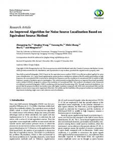
Fig 1 shows a surface with the individual manifold, before
Σi ⊂ Ω within the image. The manifolds do not overlap
and after they have been corrupted by noise. A sample input
and the boundaries between individual manifolds may be non-
image consists of four sub-surfaces, as follows: The task is to
differentiable and discontinous. The image is represented as a
process the image data to remove the noise and identify the
dataset z(x, y)∀(x, y) ∈ Ω, sampled at fixed intervals on the
constituent manifolds.
X and Y planes at a given resolution. The data is corrupted by a Gaussian noise pattern with a known variance.
Clearly, we are dealing with a combination of two separate problems here. One is to remove the point noise in the input
We wish to recover the original manifolds which consti-
data, with minimal distortion to the original data sequence,
tute the composite image, both in terms of the polynomials
which may contain structural breaks and discontinuities. The
fi (x, y) ∈ C(n), corresponding to the ith manifold and its
second is to identify the boundaries of the individual con-
domain Σi . N, the maximum order of the polynomial fi () is
stituent sub-surfaces or manifolds and recover the original
an input to the algorithm.
model. The first task is covered widely in the field of image
In this paper, we have identified a novel technique to
reconstruction or inversion which refers to the conversion of
simultaneously remove noise and recover the underlying struc-
a 2-D sample and reconstructing the original three dimen-
tural information for a noisy image and have described the
sional visual domain which created the image. In case of
implementation of the same. We believe that the two functions
images, the z data is typically luminosity/chromaticity data
are complementary to each other and we use information
and the sample points represent the pixels which compose
from one to improve the other. We show that we achieve
the image. The problem is well-studied in literature, and
2
frequencies in which no useful information is present. In other cases where the noise is closely tied to the signal itself, we can use a Kalman-Bucy filter or other kinds of structure based filtering. The problem in our current case is the presence of discontinuities in the original data itself. Discontinuities, when mapped to the spectral domain, result in very high frequency signatures which will almost certainly be eliminated in any noise filtering approach and can also confuse a tracking approach such as a Kalman filter. Clearly, we need a mechanism which can utilize the structural information about the domain to do a more intelligent noise elimination. Structural information could include direction, continuity and any others specific to the domain. In our current problem, the key information is Fig. 1.
Original manifolds making up image
that discontinuities occur over continuous lines which form the boundaries between two planes. 1) Tikhonov Regularization: In computer vision, the noise
has been identified as an “ill-posed” regularization problem
removal problem is known as the regularization problem.
[Marroquin,Mitter,Poggio88].
A regularization problem tries to find the actual data z
The problem of recovering the original model g, from a set
from a noisy sample y by a linear transformation A. i.e.
of measurements z = g(x, y) on a certain domain (x, y) ∈ D
y = Az. In the standard form given by Tikhonov, we
is related to the problem of inversion [Tarantola]. However,
solve a global optimization problem to find z such that
inversion holds the relation g constant and tries to find the
k S(z, y) k + λk P (z, y) k is minimized [Terze88]. S and
original model parameters (x, y). If g is a linear operator G,
P are domain specific stabilizing and regularizing functionals
then we can treat the coefficients of G as the model and (x, y)
respectively, based on known properties of the surfaces we
as the mapping operator, which makes it a standard inversion
are trying to reconstruct. The first term corresponds to the
problem.
deformation energy of the surface as a whole (caused by
2
2
Our problem requires an application of two separate meth-
internal discontinuities, creases and surface variations), the
ods from two related but different domains. Inversion prob-
second term gives the penalty of deviation from the original
lems don’t deal with discontinuities and structural breaks and
data. There are many forms for S and P , each with its own
require a good apriori estimate of the model. Noise erasure
complexities. Once S and P are selected, the problem has to be
problems on the other hand, do deal with discontinuities, but
solved using some form of global optimization, for example,
don’t give or use any apriori information. In our solution
simulated annealing. The challenge is to find the form of S
we have used an iterative technique which alternately uses
and P which matches our specific domain and then choosing
noise reduction and inversion to gradually build up apriori
a suitable technique for global optimization of z as per the
information about the model.
equation given above.
A. Noise reduction and smoothing
A key parameter in this equation is λ(i,j) , which gives the relative weightage between the stabilizing functional and the
Noise reduction or removal is a standard problem of data
regularizing function. The higher the value of λ, the higher the
processing and is typically solved by some form of low-
local stiffness i.e. penalty given for departure from the original
pass/band-pass filtering. This takes into account the fact that
value. We call λ(i,j) the noise quotient, because it is tied to
the noise signal is typically a wide-band process and will show up at multiple frequencies. If we have a reasonable idea of the
the properties of the noise signal i, j. 2) Controlled Continuity Surface modeling: A form of the
nature of the underlying data i.e. its spectrum, a bandpass filter
Tikhonov regularizer is given by Terzepoulos [Terze88] using
can be appropriately defined to get rid of noise by eliminating
the continuity control functions ρ(x, y) and τ (x, y), along with
3
a fixed discrepancy penalty tied to the known variance of the noise signal. It is his interpretation of the continuity control which is most interesting. Terzepoulos suggests a stabilizing functional as follows: Z Z 1 2 2 2 S= ρ(x, y){τ (x, y)(vxx + 2vxy + vyy ) 2 Ω + (1 − τ (x, y))(vx2 + vy2 )}dxdy ρ(x, y) ∈ [0, 1]∀(x, y) ∈ Ω τ (x, y) ∈ [0, 1]∀(x, y) ∈ Ω
the following energy function: Eφ (x, y, h, v) =
1 X (xi,j − zi,j )2 2σ 2 i,j X +α (hi,j + vi,j ) i,j
X +µ (xi,j − xi,j−1 )2 (1 − hi,j ) i,j
X +µ (xi,j − xi−1,j )2 (1 − hi,j ) i,j
hi,j and vi,j are the previously mentioned functionals which indicate whether there is a discontinuity on the horizontal
Here ρ(x, y) controls the continuity requirements for
and vertical axes. α is the cost of creating a discontinuity.
smoothing. As ρ(x, y) approaches zero, the penalty due to lack
The authors describe an algorithm to simultaneously compute
of continuity is reduced. As it approaches 1, the requirement
an optimal xi,j ∀i, j and also identifying the discontinuity
for continuity increases. It therefore represents the forces
points. The biggest downside to the algorithm is in the cost
of cohesion. Further, τ (x, y) forces the choice between C 0
of inverting a very large, albeit pentadiagonal matrix. The
continuity and C continuity as well as continuity of the first
author’s own solution suggests a neural network model for
order derivatives. [1 − τ (x, y)] thus represents the forces of
doing this inversion.
1
Once again, we note the dependence on the selection of
surface tension. For practical application of this method, we need to have a
hi,j and vi,j . Interestingly, [Figueiredo and Leital] does not
method computing τ and ρ at each point (x, y). Terzepoulos
provide any domain specific method to choose h and v. Instead
suggests an analogue with the physical world, by considering
the algorithm treats the vectors v and h as parameters to the
the image as a thin plate or membrane. The bending moment
optimization algorithm and estimates them indirectly.
M (x, y) = − 4 (x, y) at a point measures the local deforma2
4) Anisotropic Diffusion: Anisotropic diffusion is a version
tion energy and the divergence G(x, y) = k 5u k . [Terze88]
of the kind of global optimization attempted in simulated tear-
suggests setting τ and ρ as binary variables. τ (x, y) is set to
ing, suggested in [Perona and Malik90]. Anisotropic diffusion
1 if the bending moment at that point is greater than a pre-set
attempts to identify individual sub-surfaces by solving the heat
threshold. Similarly, ρ is set to 1 if G(x, y) is greater than a
diffusion equation
preset threshold. 3) Simulated Tearing: Simulated tearing, suggested by
∂I = c(x, y, t)4I + ∇c∇I ∂t
(1)
[Figueiredo and Leital] is a conceptual modification of sim-
where I is the intensity and c is the heat diffusion coefficient.
ulated annealing, and a further expansion of the bending
The authors suggest sub-surface identification by using an
membrane formulation suggested by [Terze88]. The simulated
appropriate formulation of c, ensuring that heat diffusion
tearing process is similar to taking a membrane or some kind
coefficient is zero on an edge and maximum within a sub-
of flexible paper and pressing it down onto the surface below.
surface. A suggested formulation by the authors for a 2-d grid
The membrane will be impervious to noise at individual points
as we use is given by:
i.e. it will deform itself to ’smoothen’ them out. However, where there is an actual discontinuity at the boundary between two or more sub-surfaces, the membrane will tear. In the final analysis, the membrane should tear into multiple pieces, each of which corresponds to a given manifold and whose orientation describes that of the manifold itself. The simulated tearing algorithm, similar to the simulated annealing algorithm, requires the construction of a suitable energy function. In [Figueiredo and Leital], the authors use
I t+1 = I t + λ{cN ∇IN + cS ∇IS + cE ∇IE + cW ∇IW } 1 ) cN,S,W,E = ( k∇IN,S,W,E k 2 ) 1+( K ∇IN = Ii−1,j − Ii,j ∇IS = Ii+1,j − Ii,j ∇IW = Ii,j−1 − Ii,j ∇IE = Ii,j+1 − Ii,j
4
The interested reader will note that the surface tension and
III. A B RIEF REVIEW OF THE INVERSION PROBLEM
adhesion parameters in this formulation is nothing but the first
In a linear inversion problem, the data parameters z, which
derivatives around each point. This paper focusses more on the
are the observation coordinates in our case, are related to the
iterative approach of solving the optimization problem as an
model parameters x, y by a function g which is constant over
evolving heat diffusion.
the x, y, at least locally. In our case, we write the relation as Z = XG, where Z = {z0 , z1 , . . . , zn } is the observation
B. An explicit two stage approach
vector, the model parameters are coefficients of the linear
A fairly simple and usable approach has been suggested by [Schunk and Sinha92]. We found the approach appealing because it is simple and simultaneously addresses the dual issues of removing noise as well as identifying surfaces. We have recreated the approach and used it reasonably successfully as we shall describe below, to generate benchmark data, against which we have validated our own algorithm. The algorithm is a two-stage method. The first stage is a noise-reduction stage. It divides the surface into small subsurfaces and try to do an optimal plane fit on each sub-surface. An innovation was to use a robust method (MLMS), which also handles the cases where individual points are corrupted with noise, as follows 1) Instead of taking all the points within the sub-surface, the algorithm randomly picks out a sub-set of the points 2) Using the sampled points, the algorithm using a fitment algorithm to fit the point selected onto a sample curve. 3) Based on the results, the algorithm computes and stores the mean square error for the sample 4) This process is done repeatedly. For each sample, the MSE is stored 5) Finally, the sample with the median MSE is chosen to represent the sub-surface. After this first step, we will have planar fits for each small sub-surface of the entire grid. This is known as the clean and fit stage. This phase is followed by the global optimization stage. The global optimizer uses a global energy function constructed out of B-splines over the basic sub-surface as follows: Z n X T (f ) = (yi − fj (xi ))2 + w(x)[f 00 (x)]2 dx i=1
operator G, and the mapping function is matrix of the form x0 y0 x0 2 y0 2 1 x1 y1 x1 2 y1 2 1 X= . .. .. .. .. .. . . . . xn yn xn 2 yn 2 1 where (x0 , y0 ), (x1 , y1 ), . . . , (xn , yn ) are the points over which the plane is being constructed. The generalized least squares technique is an accepted method of solving this problem, though it is nearly impossible to justify that the coefficients of G are sampled from a gaussian mean pdf with a known covariance vector. However, if we have existing ˆ it is not unreasonable to consider that G − G ˆ is estimates G, a gaussian in Rn and use the least squares algorithm. IV. T HE ALSD ALGORITHM As described by various researchers, and in our own estimates, the critical choice in any form of solution of the image inversion problem is the trade-off between the adhesion and tension terms respectively. As we can see from the different algorithms given above, each algorithm suggests a different method for selecting it. The proposed ALSD algorithm is a departure from the algorithms studied above, because it uses the knowledge of existing manifolds to determine whether a point is within a manifold or on a boundary, instead of using purely local information from the point i.e. its gradient or divergence, as in the examples above. Since the underlying manifolds which are themselves not necessarily flat, so the divergence for a point is not necessarily an indicator of
(2)
Ω
tension. Instead, it uses an approach of actively discovering the constituent manifolds and measuring the tension/adhesion
The key advantage that we found in this method is the
of each point with respect to the manifold in which it is
explicit attention to removing point error (cleaning) before
(possibly) situated. In this respect, it is somewhat similar to
attempting the global optimization. We have recreated it to
the first stage of [Schunk and Sinha92]. However, whereas
an extent in our own approach. A second feature, which we
[Schunk and Sinha92] uses a fixed neighbourhood of a point
have also used, is the use of local linear fit as an indicator of
purely as a way of measuring discontinuities, we all the
the deformability of the data at a point. We shall discuss this
neighbourhood to dynamically grow into a full manifold.
point further below.
This allows our algorithm to work nearly completely without
5
any heuristics and without any domain-specific, user-supplied
the ith manifold and the goodness of fit of all points
constants; instead, it adapts to the quality of the data and finds
(x, y) mapped to it, we compute a tension energy as the
the best underlying structural representation, as well as the
residual sum of squares over the domain of the manifold. X di = (fi (x, y) − z(x, y))2 (3)
likely noise term. We will now discuss the algorithm in more detail. Let us
x,y∈Si
recall the problem statement first. As given II, we have a set of
7) If a point is not mapped to a contour, we associate a
sampled data z, which is represented by a set of polynomicals P fi (x, y) in the form z = i fi (z, y)I{(x,y)∈Σi } where Σi are S disjoint sets such that i Σi = Ω. The polynomials fi (x, y)
deformation energy to it as the absolute distance from 8) The aggregate energy for the membrane is given as the
are not known initially but have to be estimated as part of
sum of the energies (both deformation and tension) for
the problem. This is further corrupted by a noise process of
all manifolds and unmapped points in the data-set
independent variance σ, which is input to the algorithm. Our algorithm works by choosing the successively running the manifold selection function, parameterized by the maximum tolerance of each manifold as discussed below. 1) Start with the input data set z0 . Identify the component manifolds and their associated ranges, so that each sample point (x, y) in the image space Ω is mapped to a one manifold. The maximum tension in a given manifold is bounded by below by the parameter T . This tension is measured as 1.0 − exp(−err(Σi , fi )), where the function err(A, f ) measures the mean square error for all the points in set A with respect to the defining polynomial f . 2) A point is mapped to a manifold if, by including it in the manifold, the tension of the manifold overall is lower than the parameter T . Thus, whether a point is
the mean height of the entire membrane
9) The algorithm is run with different values of the deformation parameter T and the best solution is taken. It is fairly clear that: a) As T drops, the number of points not mapped to a contour will drop b) As T drops, the deformation in a contour goes up, since it accepts points with higher mean square error c) At some value of T , an optimum will be achieved. We have implemented a gradient search algorithm to compute the optimal value of T d) Thus the global optimization problem becomes a search for optimal T over a convex domain. We can use a binary search or any other algorithm to find the optimal T and the corresponding set of manifolds Σi corresponding to this T .
on a boundary or not is a function of both the point
10) When the final manifolds are recovered, each point
and the manifold to which we are trying to map it.
z{x,y} 7→ {Σp , fp } is projected onto the constituent
This is the principal innovation in this algorithm; instead
manifold to get the “cleaned image”. zˆ{x,y} = fp (x, y)
of using purely local information as in [Terze88] or [Perona and Malik90], we utilize the overall fitment of the point within a particular region.
A. The manifold identification algorithm To identify individual manifolds we propose an algorithm
3) When the tension threshold is close to 1, many points
for edge detection using a localized searching technique. In
may not be mapped to any manifold, since the noise
our case, we start with an initial small set of points and start
value causes too high an error
growing a smooth manifold defined over this initial set. At
4) On the other hand, as the threshold drops towards zero,
each step, we note not only the manifold coefficients, but also
points will get mapped to manifolds even if the resultant
the distortion in the manifold caused by the constituent points.
error and consequently, surface tension of the manifold
The distortion of the manifold is checked by fitting it onto a
is high
smooth polynomial in n dimensions using a best-fit algorithm.
5) The surface tension energy plays the role of the defor-
The quality of the fitment is verified by measuring the mean
mation term in our algorithm. The parameter T plays
square error between the data set and the smooth surface. The
the role of the stabilizing function.
domain of the manifold is improved and grown by absorbing
6) Based on the associated manifold function fi (x, y) for
points around the edges of the current manifold, and also
6
eliminating points which increase the distortion. The distortion
Here, W (x) is the neighbourhood of the point x.
is limited by the parameter T , supplied to the algorithm (see
5) Now go back to step 3
above).
6) The manifold Σi,t is declared complete if R = ∅ i.e.
For a given point, the induced strain caused by it is measured as ∆e, the difference in the average MSE in the manifold with and without that point. The probability of adding the point is given by
d(e) exp(− ∆eN ), Ni
there are no points which can be added to S. 7) Continue this procedure till the entire grid is completed and it is not possible to create any further manifolds.
where Ni is the number of points
8) Now evaluate all those points which are not an ele-
in the manifold at the current time and N d(e) is the number
ment of any manifold and mark them outliers. Use any
of points in the manifold which are immediate neighbours of
smoothing function to filter out outliers.
the current point. Since it is expected that boundary points are continuous, the algorithm is more likely to reject a point if it has a neighbour which is also rejected. Points are isolated in the same manner. Individual points which have high noise will be rejected and the algorithm will grow the manifold around them, leaving them as isolated unmapped points. The local search stops when no further points can be added to a manifold. This will typically happen when there are a number of neighbouring
The principal advantage of this algorithm is that it is possible to honour exact boundaries and it is computationally relatively cheap. The principal cost of computation is the repeated cost of executing the curve-fitting algorithm. The number of times the curve-fitting must be executed is roughly of the order of the number and length of the edges in the grid. In this regard, it is roughly of the same order of complexity as the first stage of the two-stage algorithm suggested by [Schunk and Sinha92]
points spanning a border of the manifold, all of which are rejected by the local search. This set is naturally identified as the boundary.
B. Finding the locally best fitting surface As stated above, we used a least squares technique to
The algorithm is as follows: 1) Select a local manifold within the overall grid defined over an initial domain Σi,0 . Choose points in Σi,0 so that they are connected and are not currently mapped to any existing manifold (discovered previously) 2) At every iteration, use a curve fitting LMS algorithm to find the best-fitting polynomial f (Σi,t ) in the chosen number of dimensions over this manifold. Store the associated error ²(N (Σi,t ), Σi,t ) 3) Randomly select a point p ∈ Σi,t in the manifold and use the rejection metric i.e. ∆e = ²(f (Σi,t − p), Σi,t − p) − ²(f (Σi,t ), Σi,t ) r = rand() ∆e if (r > exp(− f (Σ )) remove point from manifold i,t )
else retain point in manifold 4) Once all points within the manifold S has been checked out, add a ring of points R to this manifold. A ring
estimate the best coefficents of the manifold function fi (). We experimented with two possible methods. One was the standard generalized linear regression using the Golub Reinsch singular value decomposition method. Here, there are four variables, x, y, x2 and y 2 . We used rank decimation to determine when the model was over-specified. The second technique tried was a non-linear fitting method, using the Levenberg-Marquardt transform. Both techniques proved reasonably robust in the face of errors. One of the problems in the overall algorithm is that the data presented to the curve-fitter may have structural breaks. This happens when the initial starting set is incorrectly chosen in such a way that it overlaps two or more contours. Unfortunately, neither of the considered methods are able to natively detect structural breaks; we are thus forced to rely on the residual sum of squares method and the estimated χ2 value to detect a structural break.
comprises a set of points which have at least one
The accuracy of reconstruction of the constituent polyno-
immediate neighbour which already an element of the
mials is a function both of the noise and the nature of the
existing manifold.
polynomial itself. Since the values of x and y are very small,
R = {x 6∈ Σi,t
[ Σi,t+1 = Σi,t R \ : W (x) Σi,t 6= ∅}
most of the surface fitting algorithms we tested (weighted linear fit, nonlinear Levenburg-Marquardt transform) were unable to compute the coefficients for the square terms.
7
Fig. 2.
Original Surface
V. E XPERIMENTAL DATA We started with the following original surface. The figure is generated using the following four manifolds, defined over the associated regions as given below. 1) f1 (x, y)
=
2.3x − 2.2y + 2.92x2 + 2.67y 2 +
Fig. 3.
Analysis of clean data, original and processed
Fig. 4.
Analysis of slightly noisy data, original and processed
2.455∀{(x, y) : 0 < x < 0.3, 0 < y < 0.2} : Manifold 1 2) f2 (x, y) = −1.26x + 1.11y − 1.08x2 − 1.04y 2 − 1.234∀{(x, y) : 0 < x < 0.4, 0.2 < y < 0.5} : Manifold 2 3) f3 (x, y) = 5.8∀{(x, y) : 0.4 < x < 0.5, 0 < y < 0.5} : Manifold 3 4) f4 (x, y) = 3.13x + 0.81y + 3.02x2 + 1.02y 2 + 6.2∀{(x, y) : 0.3 < x < 0.4, 0 < y < 0.2} : Manifold 4 Note
that
Ω
is
defined
over
x, y : 0