Nebojša M. Nikolić Teaching and Research Assistant University of Novi Sad Faculty of Technical Sciences
Tripo M. Torović Professor University of Novi Sad Faculty of Technical Sciences
Života M. Antonić Teaching and Research Assistant University of Novi Sad Faculty of Technical Sciences
Jovan Ž. Dorić Teaching and Research Assistant University of Novi Sad Faculty of Technical Sciences
An Algorithm for Obtaining Conditional Wear Diagram of IC Engine Crankshaft Main Journals Since crankshaft main journals belong to a group of highest loaded engine parts, it is very important to know forces acting on them. If a polar load diagram for each main journal is known, then the forces are fully defined. Using polar load diagrams, a conditional wear diagram for each main journal can be constructed, with a help of which one can predict how their surfaces are worn around the circumference. The authors have developed an algorithm for obtaining conditional wear diagrams of main journals, observing a crankshaft as a statically indeterminate continuous beam. The essence of the algorithm, tailored to its software implementation, has been shown in the scope of the paper. The authors have also performed the implementation by creating appropriate computer programs. The programs have been applied on the example of a six-cylinder diesel engine crankshaft and the results obtained are given in the paper. Keywords: crankshaft, main journal, conditional wear diagram, statically indeterminate method.
1. INTRODUCTION
The majority of common mechanical systems include relative motion between the contacting elements. The movement can be translatory and rotary. Rotary movement is in machinery more frequently used than translatory one, usually in the form of rotating shafts in their bearings or rotating pins in revolute joints [1]. Among other phenomena, the movement can be a source of wear that is usually classified as a permanent loss of the material [2]. Wear is affected by many parameters such as forces acting between the elements coupled, geometry and temperature of contact, physical and chemical properties of the contacting materials etc. It is very difficult to understand and describe the wear phenomenon, especially if all the possible physical and chemical influence parameters are taken into account. A large amount of articles has been presented over the last decades showing how wear in mechanical systems is of great importance. Flores [3] has developed a methodology for studying and quantifying the wear phenomenon in revolute clearance joints exposed to dry friction taking into account the geometry and material properties of the elements coupled. Mukras [4] compared two procedures for prediction of the revolute joint clearance evolution caused by wear. The subject of interest in this paper is a crankshaft main journal that, together with its bearing, carries the highest mechanical load in an IC engine. In addition, the load changes significantly during one engine cycle. Therefore, the forces acting between main journals and their bearings can be considered the most important factor affecting the wear of the elements in contact. Received: August 2011, Accepted: October 2011 Correspondence to: Nebojsa Nikolic Faculty of Technical Science, Trg Dositeja Obradovica 6, 21000 Novi Sad, Serbia E-mail:
[email protected] © Faculty of Mechanical Engineering, Belgrade. All rights reserved
An algorithm for constructing a conditional wear diagram of the crankshaft main journals is given in the paper. The conditional wear diagram is a visual representation of a main journal load in the form of a worn out journal, taking into account the dominant wear influence factor only – the forces acting on the journal. The forces are determined by a method treating a crankshaft as a statically indeterminate continuous beam [5]. As far as the authors are aware, there are no articles showing such an algorithm for constructing a conditional wear diagram of main journals. Some papers give graphical, less accurate procedures [6,7] and some give analytical ones [8] but in all of them a crankshaft is treated as a statically determinate beam. 2. DETERMINATION OF MAIN JOURNAL LOAD
Construction of a main journal conditional wear diagram requires a prerequisite to be fulfilled: direction and magnitude of the forces acting on the journal throughout the engine cycle have to be known. The forces are thoroughly defined by a polar load diagram that is thus the source of input data for obtaining a conditional wear diagram. Gas forces and inertia forces of crank gear elements are dominant ones and are taken into account in determining a main journal load [9,10]. Crankshaft is considered more realistically, as a statically indeterminate continuous beam carrying the forces mentioned. That means the clearances between the journals and the bearings are taken into account and consequently the crank forces are distributed to all the bearings, not only to the adjacent ones (Fig. 1). This is the main assumption upon which a construction procedure of the main journal polar load diagram is based. The authors have developed the procedure earlier, so only its essence is given here. More details are available in the reference [5]. Since all the crank forces affect all the supports, it is necessary to express the influences quantitatively. The FME Transactions (2011) 39, 157-164 157
coefficients ρ1, ρ2, …, ρn + 1 given in Figure 1 are used as a measure of the influences.
the first case considered was the one, when a unit point force acts in the middle of the span 1 (Fig. 4).
Figure 1. Main bearings load distribution according to statically indeterminate methods
2.1 Determination of influence coefficients
In order to determine the influence coefficients, a crankshaft is considered as a statically indeterminate continuous beam of constant cross-section (Fig 2).
Figure 3. Decomposition of a statically indeterminate continuous beam into the simple beams system
Figure 2. Crankshaft as a statically indeterminate continuous beam
If a crankshaft has (n + 1) main bearings and n cranks, the counterpart beam will have (n + 1) supports and n spans between them accordingly. Supposing that a point force of the magnitude 1 (unit point force) is applied vertically in the middle of the beam span i, the support reactions represent the influence coefficients required. Taking into account that a beam has n spans and (n + 1) supports, it is clear that n (n + 1) influence coefficients should be calculated. The calculation is performed using Clapeyron’s equation (the three-moment equation). A continuous beam is transformed into the system of n simple beams by the intersection method (Fig. 3). Influences of the removed parts of the original beam are compensated here by couples of moments over the supports. Supposing that the beam is of constant crosssection, Clapeyron’s equation has the form [11] M k −1lk + 2 M k (lk + lk +1 ) + M k +1lk +1 = ⎛ ⎞ = −6 EI ⎜ ∑ αs + ∑ βs ⎟ ⎜ ⎟ k ⎝ k ⎠
(1)
where: Mk – 1, Mk and Mk + 1 are moments over three consecutive supports k – 1, k and k + 1; lk and lk + 1 are lengths of the spans k and k + 1; I is moment of inertia of the beam, E is modulus of elasticity of the beam material; ∑ αs + ∑ βs is algebraic sum of the elastic k
k
curve slopes at support k due to active forces applied in the spans adjacent to the support. If one Clapeyron’s equation is written for each pair of adjacent spans of the beam with (n + 1) supports, then (n – 1) Clapeyron’s equations should be written. Calculation of the influence coefficients is equivalent to determination of the continuous beam support reactions when a unit point force is applied in the middle of a beam span, as above stated. In accordance with it, 158 ▪ VOL. 39, No 4, 2011
Figure 4. Unit point force applied in the first span of a statically indeterminate continuous beam
The system of (n – 1) Clapeyron’s equations written for the case is:
3l12 8 M1l2 + 2M 2 (l2 + l3 ) + M 3l3 = 0 ....................................................... M i −1li + 2 M i (li + li +1 ) + M i +1li +1 = 0 ....................................................... M n −3ln − 2 + 2M n − 2 (ln − 2 + ln−1 ) + M n −1ln −1 = 0 M n − 2ln −1 + 2M n −1 (ln −1 + ln ) = 0 . (2) 2M1 (l1 + l2 ) + M 2 l2 = −
If a point force F is applied in the middle of a simple beam of length l and moment of inertia I, then algebraic sum of the elastic curve slopes at the supports is Fl2/16EI [11], where E is modulus of elasticity of the beam material. Taking into account this and (1), the right-hand term in the first Clapeyron’s equation of the system (2) becomes −3l12 8 . The right-hand terms in other Clapeyron’s equations are zeros, because there are no active forces in the corresponding beam spans. When a unit point force is applied in the middle of the span n of the continuous beam, the situation is similar (Fig. 5). The difference is that the right-hand term is now zero in all the Clapeyron’s equations except in the last one where it has the value −3ln2 8 .
Figure 5. Unit point force applied in the last span of a statically indeterminate continuous beam
FME Transactions
In cases when a unit point force is applied in the interior spans of the beam, there are always two Clapeyron’s equations with right-hand terms different from zero, and the rest ones have zero at the right hand side. For example, if a unit point force is applied in the span 2 (Fig. 6), then the elastic curve slope due to the force will appear in 1st and 2nd Clapeyron’s equations.
Figure 6. Unit point force applied in the span 2 of a statically indeterminate continuous beam
are taken into account in a dynamic analysis of every IC engine. This paper is not an exception and the forces considered have been determined in a common way: gas forces according to Grinevetsky-Mazing method [6], and inertia forces using Newton’s second law of motion. After that, the connecting rod force Fcrod and the inertia force of the crank Ficrnk have been determined also in a common way [6], so that part of the calculation has not been given in the paper. In order to determine the forces acting on main journals, a crankshaft of a six-cylinder in-line engine has been analyzed (Fig. 7), but the analysis and expressions obtained are valid for all in-line engines.
Similarly, if a unit point force is applied in the span 3, then the right-hand terms in 2nd and 3rd equations are −3l32 8 , and in the others they are zeros etc. Thus n systems of Clapeyron’s equations are obtained, because there are n cases of unit point force acting in a beam span and each case is described by one equation system. Each system consists of (n – 1) equations with (n – 1) unknowns, which means that it can be solved by any of the methods known. A matrices method is used here and thus the moments over the beam supports are calculated. Knowing the moments and using the equations of the form ΣM = 0 for each simple beam, the support reactions of the continuous beam, and at the same time the influence coefficients, can be determined. There are n spans where a unit point force can be applied and (n + 1) beam supports, which means that n (n + 1) influence coefficients can be calculated as described above. The influence coefficients can be expressed in a matrix form: ⎡ ρ1,1 ⎢ ⎢ ρ 2,1 ⎢ . RO = ⎢ ⎢ ρi,1 ⎢ ⎢ . ⎢ρ ⎣ n,1
ρ1,2
.
ρi , j
.
ρ1,n +1 ⎤ ⎥
ρ2,2 . ρ 2, j . ρ 2,n +1 ⎥ .
ρi,2 .
ρn,2
. .
.
ρi , j
. . . ρ n, j
⎥ ⎥, ρi ,n +1 ⎥ ⎥ . . ⎥ . ρ n,n +1 ⎥⎦ . .
.
(3)
where the influence coefficient ρi,j is the reaction at support j when a unit point force is applied in the middle of the span i. The influence coefficients from matrix RO will be used at determining main journal load. A computer program has been developed in the scope of the research, which can be used to calculate continuous beam influence coefficients, regardless of the number of supports. Now, the forces acting on main journals during one engine cycle are determined using the influence coefficients from (3). An analytical procedure for determining the forces, which is convenient for software implementation, is shown below. 2.2 Analytical model of forces acting on the main journals
It has been said before that gas forces and inertia forces are dominant over other forces that load crankshaft main journals. Therefore, they are considered basic ones and FME Transactions
Figure 7. The force originating from the crank 1 of a sixcylinder engine crankshaft
First of all, the force originating from crank i, Fcrnki, is determined as a vector sum of the forces Fcrodi and Ficrnki, Fcrnk i = Fcrodi + Ficrnk i .
(4)
In Figure 7 this is shown for the crank 1 but (4) is valid for any crank. Each force Fcrnki (i = 1, 2, …, 6) can be decomposed into two mutually perpendicular components, one of which is in radial and the other one is in tangential direction with respect to the crank i (Fig. 8). This is described by the relation Fcrnk i = Radi + Tani .
(5)
To avoid confusion, the cranks 1, 2 and 3 are shown in Figure 8a and the cranks 4, 5 and 6 in Figure 8b.
Figure 8. Decomposition of the forces Fcrnki: (a) at the cranks 1, 2 and 3 and (b) at the cranks 4, 5 and 6
Further, the action of each of the forces Radi and Tani can be replaced by an equivalent force-couple system. The couple is irrelevant for the analysis and is not considered in the paper and the force crosses the VOL. 39, No 4, 2011 ▪ 159
axis of the crankshaft. The force from the force-couple system is projected onto the axes of the coordinate system OX1Y1 that is rotating together with the crankshaft (Fig. 9). The projections of the forces Radi and Tani have been labelled with RadX1i, TanX1i, RadY1i and Tan Y1i (i = 1, 2, 3). Only first three cranks have been shown in Figure 9 because the cranks 4, 5 and 6 have the same configuration.
Figure 9. Tangential and radial projections of Fcrnki (i = 1, 2, 3) projected onto the coordinate system fixed to the crankshaft
initial position (beginning of the engine cycle) and θi is angle that indicates the phase of the engine cycle in cylinder i when in the cylinder 1 the engine cycle is at the beginning. Each pair of values (FmbX1k,φ, FmbY1k,φ) represents a point in the coordinate system OX1Y1. Each point is a vector head end of the force acting on the main bearing k at the crankshaft angle φ. By connecting the points, calculated for different values of φ, a polar diagram is obtained defining the forces acting on the main bearing k during one engine cycle. However, to construct a main journal wear diagram, the forces acting on the main journal are relevant. Since (7) is defined with respect to the coordinate system OX1Y1 that is fixed to the crankshaft, it is only necessary to rotate the polar diagrams (7) by the angle 180° according to Newton’s third law of motion. In other words, the force Fmjk, by means of which the main bearing k acts on the appropriate journal, and the force Fmbk defined earlier, differs from each other only in direction. Therefore, the projections FmjX1k and FmjY1k of the force Fmjk can be calculated using the expressions FmjX 1k ,ϕ = − FmbX 1k ,ϕ
Taking into account the decomposition of the forces (Fig. 9) and the influence coefficients above determined, the expressions for the projections FmbX1k and FmbY1k of the force Fmbk have been derived. Fmbk denotes the force transmitting from the main journal k to its main bearing due to influences of all the cranks. For a crankshaft with n cranks, the expressions derived have the form:
FmjY 1k ,ϕ = − FmbY 1k ,ϕ .
(8)
Equations (7) and (8) have been implemented in a computer program that enables an automated construction of a main journal polar load diagrams for any in-line IC engine, knowing: influence coefficients, crankshaft configuration, firing order and dependence of gas forces and inertia forces on the angle φ.
n
FmbX 1k = ∑ (− ρi,k Radi sinψ i + ρi,k Tani cosψ i )
3. CONDITIONAL WEAR DIAGRAM OF A MAIN JOURNAL
FmbY 1k = ∑ ( ρi,k Radi cosψ i + ρi ,k Tani sinψ i ) (6)
Conditional wear diagrams of main journals can be constructed using their polar load diagrams. They give a natural picture of main journals load and a possibility to compare them on that basis. Furthermore, a conditional wear diagram provides a picture of wear profile around the main journal circumference, assuming that wear volume is proportional to the magnitude of forces acting on the journal [12]. Figure 10 shows a principle of conditional wear diagram construction. The forces Fmjφ acting on a main journal at different values of the crankshaft angle φ (φ1, φ2, φ3) have been shown in the form of vectors in Figure 10. The three values are arbitrarily chosen for illustration, but the procedure is applicable for all φ ∈ {1, 2, …, 720}. Magnitudes and directions of the vectors Fmjφ1, Fmjφ2 and Fmjφ3 are fully defined by a polar load diagram of the main journal observed. The dashed vector lines represent the vectors as they are taken over from the polar diagram, and the solid vector lines represent the vectors at the points on the journal circumference where they actually act. Angles α1, α2 and α3, measured with respect to the axis X1, define the points on the journal circumference where the forces Fmjφ1, Fmjφ2 and Fmjφ3 are applied, respectively. The construction of conditional wear diagram is based on the following assumptions [7]:
i =1 n
i =1
where: ρi,k is influence coefficient of the crank i on the main bearing k and ψi is counterclockwise angle between the cranks 1 and i. However, these are not the final expressions because they do not take into account that the engine cycles in different cylinders are phase-shifted mutually. Therefore, it is necessary to observe the forces Radi and Tani in accordance with it. Involving the conditions described in (6), the final expressions are obtained: n
FmbX 1k ,ϕ = ∑ − ρi,k Radi (ϕ +θi ) sinψ i + i =1
n
+ ∑ ρi,k Tani (ϕ +θi ) cosψ i i =1
n
FmbY 1k ,ϕ = ∑ ρi ,k Radi (ϕ +θi ) cosψ i + i =1
n
+ ∑ ρi ,k Tani (ϕ +θi ) sinψ i
(7)
i =1
where φ is crankshaft angle indicating the phase of the engine cycle in the first cylinder with respect to its 160 ▪ VOL. 39, No 4, 2011
FME Transactions
•
•
I – wear depth is proportional to the magnitude of the force causing the wear and is constant in the wear zone, II – angular wear zone is spread symmetrically with respect to the application point of the force, 60° on both sides as shown in Figure 10.
Fmjϕ = FmjX 1ϕ2 + FmjY 1ϕ2 .
(10)
The second term in (9) enables the application point of the force Fmjφ to be moved to the outer surface of the journal. This is essential for determining lower and upper angle limits of the wear zone (Fig. 10),
α ∈ [αϕ − 60, αϕ + 60] .
(11)
5. The conditional wear depth δφ, caused by the force Fmjφ, is calculated. With regard to the assumption I, it is adopted that the minimum value Fmjmin of the force causes minimum conditional wear depth of the value 1, δmin = 1. Further, using the same logic, the quantity δφ is calculated according to (12),
δϕ =
Fmjϕ Fmjmin
.
(12)
6. The cumulative conditional wear depth ∆α is increased by the value of δφ for each α from the wear zone, ∆α = ∆α + δϕ , α ∈ [αϕ − 60, αϕ + 60] . (13) Figure 10. Principle of conditional wear diagram construction
The forces Fmjφ1, Fmjφ2 and Fmjφ3 are drawn arbitrarily in order for the figure to be as illustrative as possible. For the same reason, the magnitudes of the vectors have been chosen to be noticeably different from each other. In Figure 10 each hatched area represents a journal material removed due to the action of only one of the forces Fmjφ, (φ ∈ { φ1, φ2, φ3}). It should be emphasized that wear depth is a conditional term here and for clarity of wear diagram it is represented as much larger than it really is. In further text it is called the “conditional wear depth” and is labelled with δφ. Another term introduced here is the “cumulative conditional wear depth”, ∆α, that describes exaggerated cumulative effect of the forces Fmjφ on the journal during one engine cycle. To enable automated construction of a conditional wear diagram, the authors have developed an algorithm given below: 1. Maximum and minimum values, Fmjmax and Fmjmin, of the force Fmjφ during one engine cycle are determined. 2. At the beginning, the cumulative conditional wear depth ∆α is set to zero – ∆α = 0 (α = 1, 2, …, 360°), which corresponds to a new, non-worn journal. 3. The crankshaft angle φ is set to 1° (start the engine cycle). 4. The point of application, defined by the angle αφ, and the magnitude of the force Fmjφ are determined according to (9) and (10), respectively
⎛ FmjY 1ϕ ⎜ FmjX 1ϕ ⎝
αϕ = atan ⎜ FME Transactions
⎞ ⎟ +180D , ⎟ ⎠
(9)
7. The crankshaft angle is increased by 1°, φ = φ + 1°. 8. Steps 4 to 7 are repeated until the end of the engine cycle is reached. 9. Initial radius r of the circle representing the main journal in the wear diagram is calculated as r = k ⋅ Fmjmax
(14)
where k is a coefficient of proportionality that can be arbitrarily chosen in order for the most acceptable drawing scale to obtain. 10. As shown in Figure 11, a new “radius of the journal”, r (α), is calculated by subtracting the cumulative conditional wear depth ∆α from the initial radius for each α ∈ {1, 2, …, 360}, r (α ) = r − ∆α .
(15)
11. By connecting the endpoints of the radii determined in (15) with a line, the new profile of a worn out main journal is obtained. That profile is the conditional wear diagram of the journal and shows a possible distribution of wear around the journal circumference, provided the assumptions adopted are met. 12. Steps 1 to 11 are repeated for the next main journal and so on, until the end of the crankshaft is reached. On the basis of the algorithm described, a computer program has been written, enabling conditional wear diagrams of crankshaft main journals to be constructed automatically for any IC engine. 4. ILLUSTRATIVE EXAMPLE
To illustrate the application of the algorithm and the computer programs developed, a diesel engine has been VOL. 39, No 4, 2011 ▪ 161
chosen since main journals of diesel engines are higher loaded than the ones of Otto engines. It is a Perkins four-stroke cycle liquid-cooled engine, most frequently used in agriculture machines, in trucks and for power generation. The basic engine data are given in Table 1, and the other data used are available in the reference [13]. Table 1. Basic engine data
Cylinder number
Value
Unit
6
–
Rated power
77.3
kW
Rated engine speed
2500
min–1
Compression ratio
17.5
–
Cylinder bore
101.6
mm
Cylinder stroke
114.2
mm
206.4
mm
1-5-3-6-2-4
–
Connecting rod length Firing order
Figure 12. Main journal 1: (a) polar load diagram and (b) conditional wear diagram
162 ▪ VOL. 39, No 4, 2011
Figure 11. Determining a worn journal profile
Figure 13. Main journal 2: (a) polar load diagram and (b) conditional wear diagram
FME Transactions
Figure 14. Main journal 3: (a) polar load diagram and (b) conditional wear diagram
Figure 15. Main journal 4: (a) polar load diagram and (b) conditional wear diagram
Conditional wear diagrams of main journals at rated engine regime have been constructed. This is done using computer programs implementing the analytical procedure developed during the research. The results obtained are given below in the form of conditional wear diagrams of the main journals 1 – 4. Wear diagrams for the main journals 5, 6 and 7 are not shown since they are almost identical to the ones for the journals 3, 2 and 1, respectively. Together with the wear diagrams, the corresponding polar load diagrams have also been shown because the former directly arise from the latter (Figs. 12-15). For illustration, several points on each polar diagram are labelled with the values of the crankshaft angle φ, showing the endpoints of the vectors Fmjφ. All the polar load diagrams in Figures 12-15 have been shown with the same axes limits and all the conditional wear diagrams have been shown in the same drawing scale. Thus the loads of the main journals can easily be compared. Besides, Figures 12-15 show which main journals are worn more and which ones less than
others. Specifically, it is obvious in the example that the wear of the outer main journals (journals 1 and 7) is less than that of the inner ones. This was expected even before the diagrams were constructed as the inner bearings have two adjacent cylinders, while each of the outer bearings has only one adjacent cylinder. Further, the conditional wear diagrams in Figures 12-15 show where on a journal circumference the wear will be more and where less intensive. It is expected that wear is more intensive on those parts of journal circumference where the forces with higher magnitudes are applied and vice versa. However, this is not always the case, which gives more significance to conditional wear diagrams. Together with polar load diagrams, they show a complete visual representation of journal loads for the engine regime chosen. This is best shown by Figures 12 and 13. Looking at the polar load diagram in Figure 12a, one could expect that the zones of the journal circumference close to the positive side of the Y1-axis (quadrants I and II) and the zones close to the negative
FME Transactions
VOL. 39, No 4, 2011 ▪ 163
side of the Y1-axis (quadrants III and IV), are exposed to heavy wear. But, the conditional wear diagram in Figure 12b predicts heavy wear only in the lower zones of the journal circumference and in the other zones it can be neglected. Similarly, according to the polar load diagram in Figure 13a, the most intensive wear is expected in quadrant I. However, the wear of highest intensity appears in quadrant IV according to the wear diagram in Figure 13b. Such cases, when journal circumference zones with most intensive wear do not entirely coincide with the ones where the forces are the strongest, could be explained in the following way. Some journal circumference zones are exposed to the forces Fmjφ of lower magnitudes but there are a plenty of such forces concentrated close to each other. Each of the forces Fmjφ causes no large wear, but cumulative effect could result in maximum wear depth. 5. CONCLUSION
Conditional wear diagrams of main journals of an IC engine crankshaft provide a clear visual representation of the journals load. With a help of the diagrams it can very easily and quickly be concluded which journals are higher loaded than others. In addition, it can be seen how a journal is loaded around its circumference. The research presented in the scope of the paper resulted in an algorithm for automated construction of the wear diagrams mentioned. The algorithm has been implemented in computer programs also developed by the authors and thus a very useful tool has been obtained. Using this tool, one can vary some important engine parameters and get appropriate theoretical wear profiles of the main journals. The results obtained could be used in analyses of how various factors affect main journal load and wear. Furthermore, the analyses could also be conducted on crankshaft main bearings, of course with some modifications of the algorithm and the programs developed, and this could be the subject of a future research. ACKNOWLEDGMENT
The paper is a part of research on the project: “Improvement of the quality of tractors and mobile systems with the aim of increasing competitiveness and preserving soil and environment”, record number TR31046, funded by Ministry of Science and Technological Development. REFERENCES
[1] Antonic, Z., Nikolic, N. and Radomirovic, D.: On the influence of a pin type on the friction losses in pin bearings, Mechanism and Machine Theory, Vol. 46, No. 7, pp. 975-985, 2011. [2] Bryant, M.D.: Entropy and dissipative processes of friction and wear, FME Transactions, Vol. 37, No. 2, pp. 55-60, 2009. [3] Flores, P.: Modeling and simulation of wear in revolute clearance joints in multibody systems, Mechanism and Machine Theory, Vol. 44, No. 6, pp. 1211-1222, 2009. [4] Mukras, S., Kim, N.H., Mauntler, N.A., Schmitz, T. and Sawyer, W.G.: Comparison between elastic 164 ▪ VOL. 39, No 4, 2011
foundation and contact force models in wear analysis of planar multibody system, Transactions of the ASME, Journal of Tribology, Vol. 132, No. 3, pp. 031604-1-031604-11, 2010. [5] Nikolić, N,. Antonić, Ž. and Dorić, J.: Comparison of two analytical procedures of obtaining crankshaft main bearing polar load diagram, IMK14 – Istraživanje i razvoj, Vol. 38, No. 1, pp. 3-10, 2011, (in Serbian). [6] Orlin, A.S. and Kruglov, M.G.: Internal Combustion Engines, Design and Strength Calculation of Piston Engines and Combined Engines, Машиностроение, Moscow, 1984, (in Russian). [7] Lukanin, V.N., Shatrov, M.G. at al.: Internal Combustion Engines, Dynamics and Design, Высшая школа, Moscow, 2005, (in Russian). [8] Radonjić, D.: Influence of IC engine operating regime on the wear process of crankshaft main journals, Tribologija u industriji, Vol. 11, No. 4, pp. 108-111, 1989, (in Serbian). [9] Köhler, E. and Flierl, R.: Internal Combustion Engines – Motor Mechanics, Calculation and Design of the Reciprocating Engines, Friedr. Vieweg & Sohn Verlag, Wiesbaden, 2006, (in German). [10] Heywood, J.B.: Internal Combustion Engine Fundamentals, McGraw-Hill, New York, 1988. [11] Timoshenko, S.P.: Strength of Materials, Part I: Elementary Theory and Problems, Van Nostrand Company, Princeton, 1955. [12] Bhushan, B.: Introduction to Tribology, John Wiley & Sons, New York, 2002. [13] Veinović, S., Kolendić, I. and Marušić, B.: Constructions of Internal Combustion Engines, Građevinska knjiga, Belgrade, 1968, (in Serbian).
АЛГОРИТАМ ЗА КОНСТРУИСАЊЕ УСЛОВНОГ ДИЈАГРАМА ХАБАЊА ГЛАВНИХ РУКАВАЦА КОЛЕНАСТОГ ВРАТИЛА МОТОРА СУС Небојша М. Николић, Трипо М. Торовић, Живота М. Антонић, Јован Ж. Дорић Главни рукавци коленастог вратила спадају у групу механички најоптерећенијих места у мотору СУС, па је веома важно познавати силе које делују на њих. Ове силе су потпуно дефинисане поларним дијаграмима сваког главног рукавца. Коришћењем поларних дијаграма могу се конструисати теоријски дијаграми хабања главних рукаваца, помоћу којих се може предвидети како се њихове површине хабају по обиму. Аутори су развили један поступак конструисања теоријских дијаграма хабања главних рукаваца, посматрајући коленасто вратило као статички неодређени континуални носач. У оквиру овога рада приказана је суштина тог поступка, прилагођеног за софтверску имплементацију. Израдом одговарајућих компјутерских програма, аутори су и спровели ту имплементацију. У раду је приказана и примена развијених програма на примеру коленастог вратила једног шестоцилиндричног дизел мотора. FME Transactions