An algorithm for the Forward kinematics of general 6 dof ... - CiteSeerX

An algorithm for the Forward kinematics of general 6 d.o.f parallel manipulators

Un algorithme pour la cinematique directe des manipulateurs paralleles generaux a 6 degres de liberte

Jean-Pierre MERLET Programme 6

N 1331, Novembre 1990

1

Resume La cinematique directe des robots paralleles a ete etudiee pour les architectures mecaniques dans lesquelles le manipulateur presente, en dehors de la base et du plateau mobile, des faces planes. Dans ce cas on sait que l'on peut se ramener, en general, a la resolution d'un polyn^ome mono-variable de degre 16. Mais la technique employee pour obtenir ce resultat ne peut se generaliser aux manipulateurs sans faces planes. Aucun resultat sur ce sujet n'existe dans la litterature que ce soit pour obtenir l'ensemble des solutions possibles ou concernant le nombre maximum de solutions. Nous proposons un algorithme permettant de trouver l'ensemble des con gurations solution et montrons que le nombre de solutions est majoree par 1320. En n nous exhibons une con gurations a 12 solutions. Abstract Forward kinematics has been studied mainly for parallel manipulators with planar faces. In this case the size of the set of equations from the inverse kinematics can be reduced from 6 to 3 and this last set can be combined into a polynomial in one variable of order 16. But this method cannot be extented to general parallel manipulators without planar faces for which there is no known results. We present here an algorithm for the forward kinematic of general manipulators and we show that the number of solutions is bounded by 1320. We present a con guration with twelve solutions.

2

1

Introduction

Parallel manipulators present a great interest for many industrial tasks due to their high positionning ability and high nominal load. Many applications has been presented in the past either for ight simulator [13] or as robotic devices [4], [3], for example with force-feedback control [12], [8], [9]. This kind of applications uses both inverse kinematics (which is in general straightforward) but also forward kinematics. The later is known to be a dicult problem from a long time [1]. The problem of the direct kinematics has been addressed for manipulators where the mobile plate is a triangle and each of the three articulation points on the vertices of the mobile plate are shared by two links. In this case Hunt [5] conjectured that there will be at most sixteen solutions and this conjecture has been proved geometrically in [10]. Then it has been noticed that for a xed set of links lengths each articulation point of the mobile plate lie on a circle which center and radius may be determined through the links lengths. Thus its position is fully de ned by one angle. By expressing the position of the three articulation points of the mobile as a function of the 3 angles and writing that the distance between these points are known quantities one get three equations in the sines and cosines of the unknown angles. Nanua [11] has combined these equations to get a 24th order polynomial in one of the unknown. Then it has been shown that the order of this polynomial can be reduced to 16, with only even power, if the lines normal to the circles and going through their centers lie in the same plane and a numerical procedure has enabled to nd many con gurations with sixteen assembly modes ([10], [2]). In [10] other cases has been considered for the position of the lines: if the lines are no more coplanar but intersect or are parallel we may nd a polynomial of order 20 and if the lines are in a general position the order will be 24. In the same paper it has been shown that it is possible to nd the direct kinematics polynomial for most of the various manipulators nd in the literature (as soon as the mobile plate is a triangle) with this analysis and an extensive study of the number of solutions has been performed. It has been noticed that the number of solutions will be bounded by 16 whatever is the number of d.o.f of the manipulator: for example both new prototypes of parallel manipulator developed at INRIA will have at most 16 assembly modes although one is a 6 d.o.f manipulator and the other only a 3 d.o.f rotational wrist. A very recent work [6] has proposed a method to nd a polynomial of order 16 in every cases i.e. a minimal polynomial. Thus this paper seems to conclude the study of forward kinematics for parallel manipulator with a triangular mobile plate. But this method cannot be applied if the manipulator's mobile plate is not a triangle. In this case the manipulator has no more planar faces. A recent work [7] has addressed the problem of a manipulator with 4 planar faces and two non-planar faces. But basically in this case the resolution consists in nding an equivalent manipulator with only planar faces. Thus, to the best of 3

y

A1

B1

(xb0 ; yb0 ; 0)

yr

(xa0 ; ya0 ; 0)

( 2

1

A6

(

0xa2 ; ya2 ; 0)

B6 (

(

0xb2 ; yb2 ; 0)

C

B5

xr B4

0xb3 ; yb3 ; 0)

5

A5

(

0xa3 ; ya3 ; 0)

A4

(xa2 ; ya2 ; 0)

3

B2

O

6

0xa0 ; ya0 ; 0) A2 (0xb0 ; yb0 ; 0) A3

B3 (xb2 ; yb2 ; 0)

x

(xb3 ; yb3 ; 0) 4

(xa3 ; ya3 ; 0)

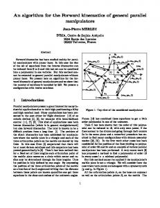
Figure 1: Top view of the considered manipulator

our knowledge, no paper has addressed the problem of the general manipulator either to nd a polynomial formulation or an upper bound of the number of assembly modes. We propose here an algorithm to nd all the assembly modes which gives also an upper bound of the number of assembly modes. This algorithm reduces the size of the set of equations to solve from 6 to 2 and we present a numerical procedure to solve this reduced set. We will consider here the case where both plates are hexagons with a symmetry axis (y and yr in Figure 1). All the articulation points Ai on the base are coplanar as well as the articulation points Bi on the mobile. The links are numbered from 1 to 6 and we de ne a reference frame (O,x,y,z) where y is the symmetry axis of the xed base. We then de ne a mobile frame (C; xr ; yr ; zr ) for the mobile with yr the symmetry axis of the mobile plate. The coordinates of the articulations point Ai in the reference frame are (xai ; yai ; zai ) and for convenience the axis z of the reference frame is chosen such that zai = 0. In the same manner the coordinates of the articulations points Bi in the mobile frame are (xbi; ybi; 0). The position of the mobile plate is de ned in the reference frame by the coordinates of point C (x ; y ; z ) and its orientation by three Euler's angles ; ;  with the associated rotation matrix R and i will denote the length of link i. The subscripts will be omitted each time there cannot be any misunderstanding. A subscript r will denote that the coordinates are expressed in the mobile frame. 0

0

0

4

2

Relation between C and R

We will consider here the expression of a links length  as a function of the position and orientation of the mobile plate. We have: AB = AO + OC + CB = AO + OC + RCBr (1) Therefore:  = AO AO T + CBr CBr T + 2(AO T + CBr T RT )OC (2) +2AO T RCBr + OC OC T The forward kinematic problem is to nd the solutions (i.e. OC and R) of a system of 6 equations of type (2) for a given set of links lengths. Let us denote dA the distance between A and O and dB the distance between B and C . These quantities are constant and are de ned by the geometry of the manipulator. Thus equation (2) can be written:  = dA + dB + 2(AO T + CBr T RT )OC +2AO T RCBr + OC OC T (3) Let us consider now two links. We de ne: Uij = dA + dB 0 dA 0 dB Wij = Ai O T 0 Aj O T Tij = CBi T 0 CBj T Sij = Ai O T RCBi 0 Aj O T RCBj We notice that Uij ; Wij ; Tij are fully determinated by the geometry of the manipulator and that the Sij are only dependent from the orientation of the robot. Let us de ne ij as: ij = i 0 j (4) Equation (4) can be written as: ij = Uij + 2Sij + 2(Wij + Tij T RT )OC (5) This equation is linear in term of the coordinates of C . If we consider the three equations  ;  ;  we get thus a linear system S in the three unknowns x ; y ; z . The resolution of this system enables to nd the coordinates of C as a function of ; ; . Thus we have: OC = H ( ; ; ) (6) Through the geometry of the problem we may notice that if a set ( ; ; ) yields to a solution (x ; y ; z ) then the set ( ; 0; ) must yield to the solution (x ; y ; 0z ). This means that for a given set of links lengths and corresponding angles we must nd the symmetrical con guration with respect to the base as a valid con guration. 2

2

2

2

2

2

i

2

i

r

2

j

j

r

r

2

12

0

0

45

0

0

65

0

0

0

0

0

5

2

r

The system S has been solved and the values of x ; y ; z are given in Appendix 1. The previous remark is satis ed during the resolution. The determinant 1 of the system is: 1 = 32sin (xa xb 0 xa xb )(sin (yb 0 yb ) + sin (ya 0 ya )) (7) which will vanished if sin  = 0, sin  = sin = 0 or sin (yb 0 yb ) = 0 sin (ya 0 ya ). In a rst step we will suppose that none of these conditions is ful lled. 0

0

3

3

0

3

0

0

2

3

2

3

3

3

2

2

The -curve

The system S being solved we may report the values of x , y , z back in the two equations  ;  . An interesting remark during this operation is that these two equations can be written as: u cos  + u = 0 v cos  + v = 0 (8) where u ; u ; v ; v contain only terms in sine and cosine of ; . These equations are described in more details in Appendix 2. From these two equations we may get an equation in ;  by writing the constraint: u v 0v u =0 (9) which yield to: p sin + p cos + (p cos + p )sin + (p sin + p )cos + sin (p cos + p ) + p cos = 0 (10) where the coecients pi are independent from . These coecients are described in Appendix 3. If we de ne x = tan equation (10) is then a sixth order polynomial in x. Let us consider this equation for a given  = s . We get then at most 6 solutions in , s ; 1  i  6. For each pair s; si equation (8) yields two solutions in , (s; 0s). Thus for a given s we get at most 6 pairs of possible solutions (s; si; s), (s ; si; 0s) which in turn yields to six pairs of solution for C , OC ; OC with: 0

24

2

1

2

1

2

2

1 2

3

1

0

36

1

1

0

2

41

3

2

1

31

32

2

42

51

2

52

6

2

i

1i

2i

OC1i

0 1 x 1 B = @ y 1 CA 0

OC2i

0

z01

i

0 1 x2 B = @ y 2 CA

(11)

0

0

z0 2

i

But by using the remark done during the resolution of the system S we know that x = x ; y = y ; z = 0z . Thus the second set of solution OC represents simply the symmetrical con guration with respect to the xed base of the rst one. Thus for every  we get at most a set of 6 possible solutions 02

01

02

01

02

2i

01

6

198

C

150

100

50

-0 0

20

40

60

80

100

120

140

160

 (degre)

Figure 2: A typical -curve ( in degree)

of the forward kinematics. They are only possible solutions because during the resolution we have used only ve equations (i.e.  ;  ;  ;  ;  ) among the set of 6 independent equations de ned by (2) and therefore we have to verify if the links lengths associated to these solutions are identical to the initial set. In order to verify the validity of a solution we de ne a performance index C : 12

C=

X 6

jjs 0 i jj i

1

45

65

24

36

(12)

where s denotes the length of link i for a possible solution. This index will vanished for each solution of the forward kinematics. By the use of a discretization of  we are able to draw a plotting of C as a function of  which is called a -curve. It is shown in Appendix 4 that the discretization of  has not to be done between [0; 2] but only between [0; ] because any solution in the range [; 2] will give identical solutions to those nd in the interval [0; ]. By looking at the -curve we can determine among the possible solutions those which have a performance index close to zero. These solutions are then fed to a least square algorithm which enables to get the exact solutions. For example if we consider the -curve described in gure 2 it appears that 4 solutions have an index close to zero. Taking into account the symmetrical solutions we will thus have 8 solutions for this particular case to which we have to add the eventual solutions corresponding to the particular cases of the resolution of the system S. i

7

4

Particular cases

The previous section does not deal with particular cases for which the determinant of the system S vanishes. First we consider the case where sin  = 0. In this case  is linear in term of x . Then  becomes linear in term of y . By using this results  can be written as z + c = 0. Thus we get two possible solutions and have only to verify if the corresponding links lengths are the same as the original set. If sin (yb 0 yb ) = 0 sin (ya 0 ya ) then equation  does not contain any term in z . It is possible to show that the -curve will be identical if we choose any other equation instead of  . Thus the only change compared with the general case is that we use another equation to compute the value of z . If sin = sin  = 0 then  is linear in term of x . Then  ;  are linear in term of y ; z . We expand  and if we de ne x = tan  we get at most fourth order polynomial in x. Thus we get a four possible solutions and have only to verify if the corresponding links lengths are the same as the original set. 12

0

34

2 0

3

2 6

0

2

3

2

65

0

65

0

0

5

12 2 1

0

0

24

65

2

Maximum number of solutions

The solution of the direct kinematic problem is the solution of the set of equations: u cos  + u = 0 (13) v cos  + v = 0 (14) (15)  ( ; ; ) =  If we de ne x = tan ,y = tan  , z = tan  this set is a set of multi-variable polynomials. The higher order term of the rst equation is x y z (term u in u ) and therefore the order of this equation is 6. The higher order term of the second equation is x y z and therefore its order is 10. The order of the last equation can be tediously found as 22 (see Appendix 5). Using Bezout's theorem we can thus state that there will be at most 6x10x22=1320 solutions. 1

2

1

2

2 1

2

2

6

2 1

2

4

4

2

2

2

2

23

2

Algorithm and Numerical example

The following algorithm has been implemented:  verify if the initial set of links lengths can satis ed the particular cases and nd the corresponding con gurations.  compute the performance index C for a discretization of  in the range [0; ] (a step of one degree seems to be sucient). 8

 if C is suciently low use the possible solution as an estimate for a leastsquare method. This algorithm has been used for a manipulator with the following characteristics: number xa ya xb yb 0 -9.7 9.1 -3 7.3 2 12.76 3.9 7.822 -1.052 3 3 -13 4.822 -6.248 The initial set of links lengths is determined for the con guration x = 05, y = 5, z = 17, = 0,  = 30,  = 0. The six over-the-base solutions are given in table 1 and the corresponding con gurations are presented in gure 3. 0

0

7

0

Conclusion

The proposed algorithm enables to nd all the solutions of the forward kinematics problem for a general 6 d.o.f. parallel manipulator. Although the computation time is rather important (about thirty seconds on a SUN 3-60 workstation) it is a rst step toward a general resolution of the dicult forward kinematics problem. The upper bound of the number of solutions is probably overestimated: we plan to continue to work on the equations to decrease it. x0

-5.0 4.8641 -10.993397 -5.0 5.502910 -4.693844

y0

5.0 3.2024 1.780824 -7.648977 -4.708340 -2.020516

z0

17.0 14.6063 12.329258 11.288760 8.390066 5.186273

0.0 323.627375 206.593364 0.0 68.130481 88.941651



30.0 95.320208 -77.993466 -118.179036 127.378302 -82.951268



0.0 36.371860 153.406322 0.0 111.871026 91.057316

Table 1: Solution of the forward kinematics problem (all the angles are in degree)

9

1

4

5

2

3

6

Figure 3: The 6 con gurations for which the links lengths are identical (perspective, top and side view). We would get the 6 others solutions by putting the mobile plate in a symmetrical position with respect to the base.

10

8

Appendix 1: Resolution of the system S

We suppose that the rotation matrix is de ned by:

0v 1 R = @ v4

v7

v2 v5 v8

v3 v6 v9

1 A

(16)

From the three equations 12 ; 45 ; 65 we are able to compute x0 ; y0 ; z0 . We get: x0 =

y0

=

z0

2 2 2 2 0 xb0 5 0 xb0 4 + 24xxb0 xS45 00 42xxb3 xS12 + xb3 1 0 xb3 2

b3 a0

b 0 a3

0xb0 xa2 25 v3 0 yb1 xb3 22v4 v3 +226 xb3 xa0 v3 0 4S65 xb3 xa0 v3 0 2U65 xb3 xa0 v3 + 4yb2 xb3 S12 v6 v1 +2yb1 xb3 S12 v6 v1 0 2S45 xb2 xa0 v3 0 2yb2 xb3 22 v4 v3 + 2yb2 xb3 21 v4 v3 0 4yb2 xb3 S12 v4 v3 02yb1 xb3 S12 v4v3 + 2xb0 yb2 25v4 v3 + 2xb0 yb1 S45 v4v3 0 2xb0 26xa3 v3 0 yb1 xa3 22v6 +yb1 xb3 22 v6 v1 0 yb1 xb3 21 v6 v1 + yb1 xa3 21 v6 + 4yb2 S45 xa0 v6 0 2xb0 yb2 24 v4 v3 +4xb0 yb2 S45 v4 v3 + 2xb0 xa2 S45 v3 + 2xb2 xa3 S12 v3 0 2xb0 S45 xa3 v3 0 xb0 yb1 24 v4 v3 +4xb0 S65 xa3 v3 + 2xb0 U65 xa3 v3 + 2S45 xb3 xa0 v3 0 2yb2 xb3 21 v6 v1 + 2xb0 yb2 24 v6 v1 02xb0 yb1 S45 v6v1 0 4xb0 yb2 S45 v6 v1 0 2xa2 xb3 S12 v3 + yb1 25 xa0 v6 0 yb1 24 xa0 v6 02xb0 yb2 25 v6 v1 + 2yb2 25xa0 v6 0 2yb2 24 xa0 v6 + 2yb1 S45 xa0 v6 02yb2 xa3 22v6 + xb0 yb1 24 v6v1 0 xb0 yb1 25 v6 v1 + xa2 xb3 21 v3 +2yb2 xa3 21 v6 0 4yb2 xa3 S12 v6 0 2yb1 xa3 S12 v6 + 2yb2 xb3 22 v6 v1 025xb2 xa0 v3 + xb0 24 xa3 v3 + yb1 xb3 21v4v3 + xb0 yb1 25 v4v3 0xa2 xb3 22 v3 + xb2 xa3 22 v3 0 24 xb3 xa0 v3 0 xb2 xa3 21v3 0xb0 xa2 24 v3 0 25xb3 xa0 v3 + 24 xb2 xa0 v3 + xb0 25xa3 v3 =8yb2 xb3 xa0 v6 v2 + 4yb1 xb3 xa0 v6 v2 0 4xb0 xa3 v6 yb1 v2 0 8xb0 xa3 v6 yb2 v2 08yb2 xb3 xa0 v5 v3 0 4yb1 xb3 xa0 v5v3 + 8xb0 xa3 yb2 v5v3 + 4xb0 xa3 yb1 v5 v3 +8ya2 xb3 xa0 v3 + 4ya1 xb3 xa0 v3 0 8xb0 ya2 xa3 v3 0 4xb0 ya1 xa3 v3 =

02xa0 ya2 25 0 2xa0 ya1 S45 0 2xa3 ya2 21 +2xa3 ya1 S12 0 4xa0 ya2 S45 + 2xa0 ya2 24 + 4xa3 ya2 S12 +4xa0 yb2 S45 v5 + 2xa0 yb1 S45 v5 0 4xa3 yb2 S12 v5 0 2xa3 yb1 S12 v5 02xa0 yb2 24 v5 0 2xa3 yb2 22v5 0 xb3 ya1 22 v1 + xb3 ya1 21 v1 +xb0 yb1 24 v5 v1 0 xa2 xb3 22 v2 + xb2 xa3 22 v2 0 25 xb2 xa0 v2 +xb0 24 xa3 v2 + yb1 xb3 21 v4 v2 0 4S65 xb3 xa0 v2 0 2U65 xb3 xa0 v2 02S45 xb2 xa0 v2 0 2yb2 xb3 22 v4 v2 + 2yb2 xb3 21 v4v2 + 2xb0 yb2 25 v4v2 02xb0 yb2 24v4 v2 + 2xb0 xa2 S45 v2 + 4yb2 xb3 S12 v5 v1 + 2yb1 xb3 S12 v5v1 02xb0 yb2 25v5 v1 + 2xb0 yb2 24v5 v1 + 2xb0 U65 xa3 v2 + 2S45 xb3 xa0 v2 +226 xb3 xa0 v2 0 2xb3 ya1 S12 v1 + 2xb0 ya2 25 v1 0 2xb0 ya2 24 v1 +4xb0 ya2 S45 v1 + 2xb0 ya1 S45 v1 + xa0 ya1 24 0 xa0 ya1 25 11

0xa3 ya1 21 + xa3 ya1 22 0 4xb0 yb2 S45 v5 v1 0 2xb0 yb1 S45 v5 v1 02xb3 ya2 22 v1 + 2xb3 ya2 21v1 0 4xb3 ya2 S12 v1 0 xb0 yb1 24 v4 v2 +xb0 ya1 25 v1 0 xb0 ya1 24 v1 + 24 xb2 xa0 v2 + 2xa3 yb2 21 v5 +2xb2 xa3 S12 v2 0 2xb0 S45 xa3 v2 0 2xb0 26 xa3 v2 + 4xb0 S65 xa3 v2 +xb0 25 xa3 v2 0 xb2 xa3 21 v2 + xa2 xb3 21 v2 0 xb0 xa2 24 v2 025 xb3 xa0 v2 + xa0 yb1 25v5 0 xa0 yb1 24 v5 0 4yb2 xb3 S12 v4v2 02yb1 xb3 S12 v4 v2 + 4xb0 yb2 S45 v4 v2 + 2xb0 yb1 S45 v4v2 + 2yb2 xb3 22 v5v1 02yb2 xb3 21v5 v1 + xb0 yb1 25v4v2 0 24 xb3 xa0 v2 + yb1 xb3 22 v5 v1 0yb1 xb3 21 v5v1 + 2xa3 ya2 22 0 xa3 yb1 22v5 0 yb1 xb3 22 v4v2 +xb0 xa2 25 v2 0 2xa2 xb3 S12 v2 0 xb0 yb1 25 v5 v1 + 2xa0 yb2 25 v5 + xa3 yb1 21 v5 =8yb2 xb3 xa0 v6 v2 + 4yb1 xb3 xa0 v6 v2 0 4xb0 xa3 v6 yb1 v2 0 8xb0 xa3 v6 yb2 v2 08yb2 xb3 xa0 v5 v3 0 4yb1 xb3 xa0 v5 v3 + 8xb0 xa3 yb2 v5 v3 + 4xb0 xa3 yb1 v5v3 +8ya2 xb3 xa0 v3 + 4ya1 xb3 xa0 v3 0 8xb0 ya2 xa3 v3 0 4xb0 ya1 xa3 v3

9

Appendix 2: Factorization of 24 ; 36

The equations (8) are of the form: u1 cos  + u2 = 0

(17) (18)

v1 cos  + v2 = 0

We have:

u1 = u11 cos  sin

+ u12 sin  cos

(19)

with u11 ; u12 constants de ned by: u11

=

04xa2 xa3 xb0 yb2 0 4xa0 xa2 xb3 yb0 + 4xa0 xa3 xb2 yb0 0 4xa0 xa3 xb2 yb3

+4xa2 xa3 xb0 yb3 + 4xa0 xa2 xb3 yb2 u12

= 4xa2 xb0 xb3 ya0 + 4xa0 xb2 xb3 ya3 + 4xa3 xb0 xb2 ya2 04xa2 xb0 xb3 ya3 0 4xa0 xb2 xb3 ya2

Then

u2 = u21 cos  sin

0 4xa3 xb0 xb2 ya0

+ u22 sin  cos + u23

with u21 ; u22 ; u23 constants de ned by: u21

u22

= 4xa2 xb0 xb3 ya0 + 4xa0 xb2 xb3 ya3 + 4xa3 xb0 xb2 ya2 04xa2 xb0 xb3 ya3 0 4xa0 xb2 xb3 ya2 =

0 4xa3 xb0 xb2 ya0

04xa2 xa3 xb0 yb2 0 4xa0 xa2 xb3 yb0 + 4xa0 xa3 xb2 yb0 0 4xa0 xa3 xb2 yb3

+4xa2 xa3 xb0 yb3 + 4xa0 xa2 xb3 yb2 u23

= 21 xa2 xb3 0 22 xa2 xb3 + 26 xa0 xb3 0 23 xa0 xb3 +22 xa3 xb2 0 21 xa3 xb2 0 25 xa0 xb2 + 24 xa0 xb2 026xa3 xb0 + 23 xa3 xb0 + 25xa2 xb0 0 24 xa2 xb0 12

(20)

Then

v1 = v11 sin2

+ v12 cos2

+ v13

(21)

with: v11 = v111 cos  + v112 sin 

(22)

where v111 ; v112 are constants de ned by: = 4xa2 xa3 xb0 yb23 0 4xa0 xa3 xb2 yb23 + 4xa0 xa2 xb3 yb2 yb3 0 4xa2 xa3 xb0 yb2 yb3 04xa0 xa2 xb3 yb0 yb3 + 8xa0 xa3 xb2 yb0 yb3 0 4xa2 xa3 xb0 yb0 yb3 0 4xa0 xa2 xb3 yb0 yb2 +4xa2 xa3 xb0 yb0 yb2 + 4xa0 xa2 xb3 yb20 0 4xa0 xa3 xb2 yb20

v111

= 4x2a0 xb0 xb3 yb3 0 4xa0 xa2 xb2 xb3 yb3 + 4xa2 xa3 xb0 xb2 yb3 0 4xa0 xa3 x2b0 yb3 +4xa0 xa3 x2b3 yb2 0 4x2a3 xb0 xb3 yb2 0 4x2a0 xb0 xb3 yb2 + 4xa0 xa3 x2b0 yb2 0 4xa0 xa3 x2b3 yb0 +4xa0 xa2 xb2 xb3 yb0 + 4x2a3 xb0 xb3 yb0 0 4xa2 xa3 xb0 xb2 yb0

v112

Then

v12 = sin v121

(23)

with v121 a constant: v121

and: and

= 4xb0 xb3 ya0 ya3 yb3 0 4xb0 xb3 ya2 ya3 yb3 + 4xb0 xb3 ya0 ya2 yb3 0 4xb0 xb3 ya20 yb3 +4xb0 xb3 ya23 yb2 0 8xb0 xb3 ya0 ya3 yb2 + 4xb0 xb3 ya20 yb2 0 4xb0 xb3 ya23 yb0 +4xb0 xb3 ya2 ya3 yb0 + 4xb0 xb3 ya0 ya3 yb0 0 4xb0 xb3 ya0 ya2 yb0 v13 = v131 sin2  + v132 v131 = v1311 sin

+ v1312

(24) (25)

where v1311 ; v1312 are constants de ned by: v1311

v1312

Then

= 4xa0 xa3 ya2 yb23 0 4xa0 xa3 ya0 yb23 0 4xa0 xa3 ya3 yb2 yb3 + 4xa0 xa3 ya0 yb2 yb3 +4xa0 xa3 ya3 yb0 yb3 0 8xa0 xa3 ya2 yb0 yb3 + 4xa0 xa3 ya0 yb0 yb3 + 4xa0 xa3 ya3 yb0 yb2 04xa0 xa3 ya0 yb0 yb2 0 4xa0 xa3 ya3 yb20 + 4xa0 xa3 ya2 yb20 0 4xa0 xa2 xb2 xb3 ya3 +4x2a0 xb0 xb3 ya3 + 4xa2 xa3 xb0 xb2 ya3 0 4xa0 xa3 x2b0 ya3 + 4xa0 xa3 x2b3 ya2 04x2a3 xb0 xb3 ya2 0 4x2a0 xb0 xb3 ya2 + 4xa0 xa3 x2b0 ya2 0 4xa0 xa3 x2b3 ya0 +4xa0 xa2 xb2 xb3 ya0 + 4x2a3 xb0 xb3 ya0 0 4xa2 xa3 xb0 xb2 ya0 = 4xa0 xb2 xb3 ya23 0 4xa2 xb0 xb3 ya23 0 4xa0 xb2 xb3 ya2 ya3 + 4xa3 xb0 xb2 ya2 ya3 04xa0 xb2 xb3 ya0 ya3 + 8xa2 xb0 xb3 ya0 ya3 0 4xa3 xb0 xb2 ya0 ya3 + 4xa0 xb2 xb3 ya0 ya2 04xa3 xb0 xb2 ya0 ya2 0 4xa2 xb0 xb3 ya20 + 4xa3 xb0 xb2 ya20 v132 = cos (q1 sin  + q2 ) + q3 sin  + q4

13

(26)

with q1 q2 q3 q4

= = = =

q11 cos

+ q12 sin sin q31 cos sin q41 sin q21 cos

The qij are constants de ned by: = 4(ya3 0 ya0 )(xa3 xb0 ya2 yb3 0 xa3 xb0 ya0 yb3 0 xa0 xb3 ya3 yb2 +xa0 xb3 ya2 yb2 0 xa3 xb0 ya2 yb2 +xa3 xb0 ya0 yb2 + xa0 xb3 ya3 yb0 0 xa0 xb3 ya2 yb0 )

q11

q12

q21

04(ya3 0 ya0 )(xa0 xa3 xb2 yb3 0 xa2 xa3 xb0 yb3 0 xa0 xa2 xb3 yb2 +xa2 xa3 xb0 yb2 + xa0 xa2 xb3 yb0 0 xa0 xa3 xb2 yb0 )

= 4(yb3 0 yb0 )(xa3 xb0 ya2 yb3 0 xa3 xb0 ya0 yb3 0 xa0 xb3 ya3 yb2 + xa0 xb3 ya2 yb2 0xa3 xb0 ya2 yb2 + xa3 xb0 ya0 yb2 + xa0 xb3 ya3 yb0 0 xa0 xb3 ya2 yb0 ) q31

q41

=

=

= 4(xa0 xb2 xb3 ya3 0 xa2 xb0 xb3 ya3 0 xa0 xb2 xb3 ya2 + xa3 xb0 xb2 ya2 +xa2 xb0 xb3 ya0 0 xa3 xb0 xb2 ya0 )(yb3 0 yb0 )

04xa0 xa3 (yb3 0 yb0 )(ya2 yb3 0 ya0 yb3 0 ya3 yb2 + ya0 yb2 + ya3 yb0 0 ya2 yb0 )

Finally v2 is de ned by:

v2 = v21 sin2

+ v22 cos2

+ v23

(27)

with: v21 v22 v23

= v211 sin  + v212 cos  = v221 sin  = g1 sin + g2 cos + g3 sin cos + g4 cos  + g5 sin 

(28) (29) (30)

with v211

v212

v221

= 4xa0 xb3 ya3 yb2 yb3 0 4xa3 xb0 ya3 yb2 yb3 0 4xa0 xb3 ya2 yb2 yb3 + 4xa3 xb0 ya2 yb2 yb3 04xa0 xb3 ya3 yb0 yb3 + 4xa3 xb0 ya3 yb0 yb3 + 4xa0 xb3 ya0 yb0 yb3 0 4xa3 xb0 ya0 yb0 yb3 +4xa0 xb3 ya2 yb0 yb2 0 4xa3 xb0 ya2 yb0 yb2 0 4xa0 xb3 ya0 yb0 yb2 + 4xa3 xb0 ya0 yb0 yb2 = 4xa0 xb2 xb3 ya3 yb3 0 4xa2 xb0 xb3 ya3 yb3 0 4xa0 xb2 xb3 ya2 yb3 + 4xa3 xb0 xb2 ya2 yb3 +4xa2 xb0 xb3 ya0 yb3 0 4xa3 xb0 xb2 ya0 yb3 0 4xa0 xb2 xb3 ya3 yb0 + 4xa2 xb0 xb3 ya3 yb0 +4xa0 xb2 xb3 ya2 yb0 0 4xa3 xb0 xb2 ya2 yb0 0 4xa2 xb0 xb3 ya0 yb0 + 4xa3 xb0 xb2 ya0 yb0 = 4xa3 xb0 ya2 yb23 0 4xa3 xb0 ya0 yb23 0 4xa3 xb0 ya3 yb2 yb3 + 4xa3 xb0 ya0 yb2 yb3 +4xa3 xb0 ya3 yb0 yb3 0 4xa0 xb3 ya2 yb0 yb3 0 4xa3 xb0 ya2 yb0 yb3 + 4xa0 xb3 ya0 yb0 yb3 +4xa0 xb3 ya3 yb0 yb2 0 4xa0 xb3 ya0 yb0 yb2 0 4xa0 xb3 ya3 yb20 + 4xa0 xb3 ya2 yb20 14

and g1 g2 g3

= g11 cos2  + g12 cos  sin  + g13 = g21 sin2  + g23 cos  sin  + g24 = g31 sin  + g32 cos 

(31) (32) (33)

where gij are constants de ned by: = 4xa3 xb0 ya2 ya3 yb3 0 4xa3 xb0 ya0 ya3 yb3 0 4xa3 xb0 ya0 ya2 yb3 + 4xa3 xb0 ya20 yb3 04xa0 xb3 ya23 yb2 + 4xa0 xb3 ya2 ya3 yb2 0 4xa3 xb0 ya2 ya3 yb2 + 4xa0 xb3 ya0 ya3 yb2 +4xa3 xb0 ya0 ya3 yb2 0 4xa0 xb3 ya0 ya2 yb2 + 4xa3 xb0 ya0 ya2 yb2 0 4xa3 xb0 ya20 yb2 +4xa0 xb3 ya23 yb0 0 4xa0 xb3 ya2 ya3 yb0 0 4xa0 xb3 ya0 ya3 yb0 + 4xa0 xb3 ya0 ya2 yb0

g11

g12

= 4xa0 xb2 xb3 ya23 0 4xa2 xb0 xb3 ya23 0 4xa0 xb2 xb3 ya2 ya3 + 4xa3 xb0 xb2 ya2 ya3 04xa0 xb2 xb3 ya0 ya3 + 8xa2 xb0 xb3 ya0 ya3 0 4xa3 xb0 xb2 ya0 ya3 + 4xa0 xb2 xb3 ya0 ya2 04xa3 xb0 xb2 ya0 ya2 0 4xa2 xb0 xb3 ya20 + 4xa3 xb0 xb2 ya20 g13

g21

g23

= 24 xa0 xb2 yb3 0 4xa3 xb0 ya2 ya3 yb3 0 21 xa0 xb3 yb3 + 22 xa3 xb2 yb3 021 xa3 xb2 yb3 0 25xa0 xb2 yb3 + 2U65 xa0 xb3 yb0 0 226 xa0 xb3 yb0 02U65 xa3 xb0 yb0 + 226xa3 xb0 yb0 0 25 xa0 xb3 yb2 0 24 xa0 xb3 yb2 021 xa2 xb3 yb0 + 22xa0 xb3 yb2 + 21 xa0 xb3 yb2 + 25 xa3 xb0 yb2 02U65 xa0 xb3 yb3 + 25 xa2 xb0 yb3 0 24xa2 xb0 yb3 0 4xa0 xb3 ya0 ya3 yb3 +226 xa0 xb3 yb3 + 2U65 xa3 xb0 yb3 0 2U24 xa3 xb0 yb3 + 24 xa3 xb0 yb2 022 xa3 xb0 yb2 0 21xa3 xb0 yb2 + 22 xa2 xb3 yb0 0 25 xa3 xb0 yb0 0 24xa3 xb0 yb0 025 xa2 xb0 yb0 + 24xa2 xb0 yb0 + 4xa0 xb3 ya2 ya3 yb3 0 2U24 xa0 xb3 yb2 +2U24 xa3 xb0 yb2 0 4xa0 xb3 ya2 ya3 yb2 + 4xa3 xb0 ya2 ya3 yb2 + 25 xa0 xb3 yb0 +24 xa0 xb3 yb0 0 22 xa3 xb2 yb0 + 21 xa3 xb2 yb0 + 25 xa0 xb2 yb0 024 xa0 xb2 yb0 0 226 xa3 xb0 yb3 0 4xa3 xb0 ya0 ya3 yb0 + 4xa3 xb0 ya0 ya2 yb0 +21 xa2 xb3 yb3 0 22 xa0 xb3 yb3 0 22 xa2 xb3 yb3 + 2U24 xa0 xb3 yb3 +22 xa3 xb0 yb3 + 21 xa3 xb0 yb3 + 4xa3 xb0 ya0 ya3 yb3 + 4xa0 xb3 ya0 ya3 yb0 +4xa0 xb3 ya0 ya2 yb2 0 4xa3 xb0 ya0 ya2 yb2 0 4xa0 xb3 ya0 ya2 yb0

= 4xa2 xa3 xb0 ya3 yb3 0 4xa0 xa3 xb2 ya3 yb3 + 4xa0 xa3 xb2 ya0 yb3 0 4xa2 xa3 xb0 ya0 yb3 +4xa0 xa2 xb3 ya3 yb2 0 4xa2 xa3 xb0 ya3 yb2 0 4xa0 xa2 xb3 ya0 yb2 + 4xa2 xa3 xb0 ya0 yb2 04xa0 xa2 xb3 ya3 yb0 + 4xa0 xa3 xb2 ya3 yb0 + 4xa0 xa2 xb3 ya0 yb0 0 4xa0 xa3 xb2 ya0 yb0 = 4xa0 xa3 ya0 yb23 0 4xa0 xa3 ya2 yb23 + 4xa0 xa3 ya3 yb2 yb3 0 4xa0 xa3 ya0 yb2 yb3 04xa0 xa3 ya3 yb0 yb3 + 8xa0 xa3 ya2 yb0 yb3 0 4xa0 xa3 ya0 yb0 yb3 0 4xa0 xa3 ya3 yb0 yb2 +4xa0 xa3 ya0 yb0 yb2 + 4xa0 xa3 ya3 yb20 0 4xa0 xa3 ya2 yb20 + 4xa0 xa2 xb2 xb3 ya3 04x2a0 xb0 xb3 ya3 0 4xa2 xa3 xb0 xb2 ya3 + 4xa0 xa3 x2b0 ya3 0 4xa0 xa3 x2b3 ya2 +4x2a3 xb0 xb3 ya2 + 4x2a0 xb0 xb3 ya2 0 4xa0 xa3 x2b0 ya2 + 4xa0 xa3 x2b3 ya0 04xa0 xa2 xb2 xb3 ya0 0 4x2a3 xb0 xb3 ya0 + 4xa2 xa3 xb0 xb2 ya0 15

g24

= 21 xb3 ya2 yb3 0 22 xb3 ya2 yb3 + 25 xb0 ya2 yb3 0 24 xb0 ya2 yb3 +22 xb3 ya0 yb3 0 21 xb3 ya0 yb3 0 25 xb0 ya0 yb3 + 24 xb0 ya0 yb3 +22 xb3 ya3 yb2 0 21 xb3 ya3 yb2 0 25 xb0 ya3 yb2 + 24 xb0 ya3 yb2 022 xb3 ya0 yb2 + 21 xb3 ya0 yb2 + 25xb0 ya0 yb2 0 24 xb0 ya0 yb2 022 xb3 ya3 yb0 + 21 xb3 ya3 yb0 + 25xb0 ya3 yb0 0 24 xb0 ya3 yb0 +22 xb3 ya2 yb0 0 21 xb3 ya2 yb0 0 25 xb0 ya2 yb0 + 24 xb0 ya2 yb0

= 4xa2 xa3 xb0 yb23 0 4xa0 xa3 xb2 yb23 + 4xa0 xa2 xb3 yb2 yb3 0 4xa2 xa3 xb0 yb2 yb3 04xa0 xa2 xb3 yb0 yb3 + 8xa0 xa3 xb2 yb0 yb3 0 4xa2 xa3 xb0 yb0 yb3 0 4xa0 xa2 xb3 yb0 yb2 +4xa2 xa3 xb0 yb0 yb2 + 4xa0 xa2 xb3 yb20 0 4xa0 xa3 xb2 yb20

g31

g32

= 4xb0 xb3 ya0 ya3 yb3 0 4xb0 xb3 ya2 ya3 yb3 + 4xb0 xb3 ya0 ya2 yb3 0 4xb0 xb3 ya20 yb3 +4xa0 xa2 xb2 xb3 yb3 0 4x2a0 xb0 xb3 yb3 0 4xa2 xa3 xb0 xb2 yb3 + 4xa0 xa3 x2b0 yb3 +4xb0 xb3 ya23 yb2 0 8xb0 xb3 ya0 ya3 yb2 + 4xb0 xb3 ya20 yb2 0 4xa0 xa3 x2b3 yb2 +4x2a3 xb0 xb3 yb2 + 4x2a0 xb0 xb3 yb2 0 4xa0 xa3 x2b0 yb2 0 4xb0 xb3 ya23 yb0 +4xb0 xb3 ya2 ya3 yb0 + 4xb0 xb3 ya0 ya3 yb0 0 4xb0 xb3 ya0 ya2 yb0 + 4xa0 xa3 x2b3 yb0 04xa0 xa2 xb2 xb3 yb0 0 4x2a3 xb0 xb3 yb0 + 4xa2 xa3 xb0 xb2 yb0

g4

= 22 xa3 ya2 yb3

g5

=

0 21xa3 ya2 yb3 0 25 xa0 ya2 yb3 + 24 xa0 ya2 yb3

022 xa3 ya0 yb3 + 21 xa3 ya0 yb3 + 25xa0 ya0 yb3 024 xa0 ya0 yb3 0 22 xa3 ya3 yb2 + 21xa3 ya3 yb2 +25 xa0 ya3 yb2 0 24 xa0 ya3 yb2 + 22 xa3 ya0 yb2 021 xa3 ya0 yb2 0 25 xa0 ya0 yb2 + 24xa0 ya0 yb2 +22 xa3 ya3 yb0 0 21 xa3 ya3 yb0 0 25 xa0 ya3 yb0 +24 xa0 ya3 yb0 0 22 xa3 ya2 yb0 + 21 xa3 ya2 yb0 + 25 xa0 ya2 yb0 0 24 xa0 ya2 yb0 2U24 xa3 xb0 ya2 0 24 xa0 xb2 ya0 0 25 xa3 xb0 ya0 024 xa3 xb0 ya0 0 25 xa2 xb0 ya0 + 24 xa2 xb0 ya0 021 xa3 xb2 ya3 + 22 xa3 xb0 ya3 + 24 xa0 xb2 ya3 025 xa0 xb3 ya2 0 24 xa0 xb3 ya2 + 22 xa0 xb3 ya2 021 xa3 xb0 ya2 + 22 xa2 xb3 ya0 + 2U24 xa0 xb3 ya3 +2U65 xa0 xb3 ya0 0 226 xa0 xb3 ya0 0 2U65 xa3 xb0 ya0

+226 xa3 xb0 ya0 + 21 xa3 xb0 ya3 + 25 xa2 xb0 ya3 024 xa2 xb0 ya3 0 21 xa2 xb3 ya0 + 25 xa0 xb3 ya0 02U65 xa0 xb3 ya3 + 226 xa0 xb3 ya3 + 2U65 xa3 xb0 ya3 02U24 xa3 xb0 ya3 0 226 xa3 xb0 ya3 0 2U24 xa0 xb3 ya2 +21 xa0 xb3 ya2 + 25 xa3 xb0 ya2 + 24 xa3 xb0 ya2 022 xa3 xb0 ya2 + 24 xa0 xb3 ya0 0 22 xa3 xb2 ya0 +21 xa3 xb2 ya0 + 25 xa0 xb2 ya0 0 22 xa2 xb3 ya3 +21 xa2 xb3 ya3 0 21 xa0 xb3 ya3 0 22 xa0 xb3 ya3 0 25 xa0 xb2 ya3 + 22 xa3 xb2 ya3 16

We notice that: u11 u12 q11 q12 v111

10

= = = = =

(34) (35) (36) (37) (38)

u22 u21 g11 g21 g31

Appendix 3: Equation 10

From the system: u1 cos  + u2 = 0

(39) (40)

v1 cos  + v2 = 0

we get the equation in the variables ; : u1 v 2

which can be expressed in

0 u2v1 = 0

(41)

by:

p1 sin3

+ p2 cos3 + (p31 cos + p32 ) sin2 +(p41 sin + p42 ) cos2 + sin (p51 cos + p52 ) + p6 cos

=0

(42) (43)

The coecients pi can be written as: =) p1 = x1 cos2  + x2 cos  sin 

(44)

with: x1 x2

= u11 v212 0 u12 v111 = u11 v211 0 u12 v112 =) p2 = x3 sin2 

where:

x3 = u12 v221

(45)

0 u11 v121

=) p31 = x4 cos2  + x5 sin2  + x6 cos  sin 

(46)

with: x4 x5 x6

= g32 u11 0 q21 u12 = u12 v211 0 u11 v112 = u12 v212 0 q31 u12

=) p32 = x7 cos3  + x8 sin  cos2  + x9 cos  sin2  + x10 cos  + x11 sin  17

(47)

with x7 x8 x9 x10 x11

and

= q11 u11 = g12 u11 0 q12 u12 = 0u12 v1311 = 0u23 v111 0 q41 u12 + g13 u11 = 0u23 v112

=) p41 = x12 sin2  + x13 cos  sin 

(48)

where x12 x13

= u12 v111 0 q31 u11 = u11 v221 0 u12 v121 + g32 u12 0 q21 u11

=) p42 = x14 sin3  + x15 cos  sin2  + x16 sin 

(49)

with: x14 x15 x16

= q12 u12 0 u11 v1312 = g23 u12 0 q11 u11 = g24 u12 0 u23 v121

=) p51 = x17 sin3  + x18 cos  sin2  + x19 sin  cos2  +x20 sin  + x21 cos 

(50)

where: x17 x18 x19 x20 x21

= = = = =

0u11 v1311 g12 u12 0 u12 v1312 g23 u11

0 q31 u23 0 q41 u11 g24 u11 0 q21 u23

g13 u12

=) p52 = x22 sin2  + x23 cos2  + x24 cos  sin  + x25 with: x22 x23 x24 x25

= 0u23 v1311 = g4 u11 = g5 u11 0 q12 u23 = 0q41 u23

18

(51)

=) p6 = x26 sin2  + x27 cos  sin 

(52)

where: x26 x27

= g5 u12 0 u23 v1312 = g4 u12 0 q11 u23

Using the tangent of the the half angle equation (42) yield to a six order polynomial: i=6 X i=0

ei xi = 0

(53)

with e0 e1 e2 e3 e4 e5 e6

11

= = = = = = =

p6 + p42 + p2

2p52 + 2p51 + 2p41 p6 0 p42 + 4p32 + 4p31 0 3p2 4p52 0 4p41 + 8p1 0p6 0 p42 + 4p32 0 4p31 + 3p2 2p52 0 2p51 + 2p41 p42

0 p6 0 p2

Appendix 4: Discretization of the -curve

We will show that the discretization on  is necessary only in the range [0,]. We notice that if [; ] is a solution of equation (53) then [ + ; +  ] is also a solution of this equation. Then we notice that: u1 ( ; ) = u1 ( + ;  + ) u2 ( ; ) = u2 ( + ;  + ) v1 ( ; ) = v1 ( + ;  + ) v2 (

0 ; ) = 0v2 (

+ ;  + )

and therefore the solution in  obtained from equation (8) are identical. If [ ; ; ], [ ; 0; ] are solutions then [ + ; ;  +  ], [ + ; 0;  +  ] are also solutions. The rotation matrix R is such that: R( ; ; ) = R( + ; 0;  +  ) which yield to:

H (( ; ; ) = H ( + ;

0;  + )

The con gurations associated to ( ; ; ), ( + ; 0;  + ) are therefore identical. In the same way: R( ; 0; ) = R( + ; ;  +  ) and therefore:

0; ) = H The con gurations associated to ( ; 0; ), ( H (( ;

( + ; ;  +  )

+ ; ;  +  ) are therefore identical. This justify that the discretization is necessary only in the range [0, ]. 19

12

Appendix 5: Order of equation (15)

We want to determine the order of the equation: 21 ( ; ; ) = 21

The left part of this equation is de ned by the norm of the vector A1 B1 . Thus we study each componant of this vector and calculate its higher order term only. 12.1

Study of

A1 B1

[1]

We have:

A1 B1 [1] =

with:

dt1 = 4(xa3 xb0

and:

nt1 dt1

0 xa0 xb3 )

nt1 = w1 sin  + w2 cos  + w3

with w3 =

cte . w1 = cos (w11 sin

+ w12 cos ) + w13 cos + w23

w2 = cos (w21 sin ) + w22 cos

with w22 = 0w11 , w12 = w23 , w13 = w21 , all these terms being constant. 12.1.1

Degree of

w1 =

A1 B1 [1]

z2 x x2 x2 x2 z 2 ( + )+ = 2 2 2 2 (1 + z ) (1 + x ) (1 + x ) (1 + x ) (1 + x2 )(1 + z 2 )

w2 =

z2 x x2 x2 z 2 + + w = 23 (1 + z 2 ) (1 + x2 ) (1 + x2 ) (1 + z 2 )(1 + x2 )

which yield to: nt1 =

x2 z 2 y 2 x2 z 2 y + + w3 (1 + x2 )(1 + z 2 )(1 + y2 ) (1 + x2 )(1 + z2 )(1 + y 2 )

therefore:

12.2

Study of

We have: with:

x2 y 2 z 2 nt1 = 2 dt1 (1 + x )(1 + y2 )(1 + z 2 )

A1 B1

[2] A1 B1 [2] = dt2 = pp1 sin

20

nt2 dt2

+ pp2 sin 

where: pp1 pp2

= 4(xa0 xb3 yb3 0 xa0 xb3 yb2 0 xb0 xa3 yb3 + xb0 xa3 yb2 ) = 4(xa0 xb3 ya3 0 xa0 xb3 ya2 0 xb0 xa3 ya3 + xb0 xa3 ya2 )

We have:

nt2 = pp3 sin  + pp4 cos  + pp5

where pp3 ; pp4 are constant. with:

pp5 = pq1 cos  + pq2

pq1 = pr1 sin2  + sin (pr3 cos  + pr4 ) + pr6 cos  + pr7

where: pr1 = ps1 sin

+ ps2 cos pr3 = ps3 sin + ps4 cos pr4 = ps5 cos2 + ps6 cos sin pr6 = ps7 cos sin pr7 = ps8 sin

in which the terms psj are constant. And: pq2 = qr1 sin2  + sin (qr3 cos  + qr4 ) + qr6 cos  + qr7

with: qr1 = qs1 sin

+ qs2 cos + qs4 cos + qs6 + qs8 sin cos + qs10 cos

qr3 = qs3 sin

qr4 = qs5 sin2

qr6 = qs7 sin2 qr7 = qs9 sin

in which the terms qsi are constants. 12.2.1

Degree of

We have:

A1 B1 [2] dt2 = pp1

which yield to: dt2 =

x

(1 + x2 )

+ pp2

y

(1 + y 2 )

pp1x(1 + y 2 ) + pp2y(1 + x2 ) (1 + x2 )(1 + y2 )

Then: qr7 = qr6 =

x2 (1 + x2 )

x3 (1 + x2 )2

21

qr4 = qr3 = qr1 =

pq2

=

x4 (1 + x2 )2 x2 (1 + x2 ) x2 (1 + x2 )

x2 y2 y2 y x2 + ( + (1 + x2 ) (1 + y 2 )2 (1 + y 2 ) (1 + x2 ) (1 + y 2 ) y2 x3 x2 x4 ) + + (1 + x2 )2 (1 + x2 )2 (1 + y 2 ) (1 + x2 )

thus: pq2 =

x4 y 4

(1 + x2 )2 (1 + y 2 )2

Then: pr7 = pr6 = pr4 = pr3 = pr1 =

x

(1 + x2 )

x3 (1 + x2 )2 x4 (1 + x2 )2 x2 (1 + x2 ) x2 (1 + x2 )

Hence: pq1

=

y x2 x2 y2 y2 + ( + 2 2 2 2 2 (1 + x ) (1 + y ) (1 + y ) (1 + x ) (1 + y 2 ) x4 x3 y2 x )+ + 2 2 2 2 (1 + x ) (1 + x ) (1 + y 2 ) (1 + x2 )

and therefore: pq1 =

This yield to: pp5 =

x 3 y 4 + x4 y 3 z2 x4 y 4 + 2 2 2 2 2 2 (1 + x ) (1 + y ) (1 + z ) (1 + x )2 (1 + y 2 )2

Hence: pp5 =

Therefore: nt2 =

x 3 y 4 + x4 y 3 (1 + x2 )2 (1 + y 2 )2

z

(1 + z 2 )

+

x4 y 4 z 2

(1 + x2 )2 (1 + y 2 )2 (1 + z 2 ) z2 x4 y 4 z 2 + (1 + z 2 ) (1 + x2 )2 (1 + y 2 )2 (1 + z 2 )

22

which yield to: nt2 =

x4 y 4 z 2 (1 + x2 )2 (1 + y 2 )2 (1 + z 2 )

The nal result is: nt2 x4 y 4 z 2 = 2 2 2 dt2 (1 + x )(1 + y )(1 + z )(pp1 xy 2 + pp2 x2 y + pp2 y + pp1 x) 12.3

Study of

We have:

A1 B1

[3] A1 B1 [3] =

where:

nt3 dt3

dt3 = sin (r1 sin  + r2 sin )

with r1 r2

Then: where:

= 4(0xa0 xb3 ya3 + xa0 xb3 ya2 + xb0 xa3 ya3 0 xb0 xa3 ya2 ) = 4(0xa0 xb3 yb3 + xa0 xb3 yb2 + xb0 xa3 yb3 0 xb0 xa3 yb2 ) nt3 = qw1 cos2  + qw2 cos  + qw3 sin2  + qw4

qw1 = qsw1 sin2  + qsw2 cos  sin  + qsw3 cos  + qsw4 sin  + qsw5

with: qsw5 = psw1 cos

sin

qsw4 = psw2 cos

qsw2 = psw4 cos2

+ psw5 cos sin + psw6

qsw3 = psw3 sin

qsw1 = psw7 cos2

+ psw8 cos sin

the terms pswi being constant. Then we have: qw2 = rw1 cos2  + rw2 cos  sin  + rw3 cos  + rw4 sin  + rw5

with: rw1 = rsw1 cos2

+ rsw2 cos sin + rsw3 rw2 = rsw4 cos + rsw5 cos sin + rsw6 rw3 = rsw7 cos + rsw8 sin rw4 = rsw9 cos + rsw10 sin rw5 = rsw11 cos2 + rsw12 cos sin + rsw13 2

in which the terms rswi are constants. Then: qw3 = tw1 sin2  + tw2 cos  sin  + tw3 cos  + tw4 sin 

23

where tw1 = cte and tw2 = cte tw3 = tw31 sin tw4 = tw32 sin

with tw31 ; tw32 constants. Finally: qw4 = yw1 sin2  + yw2 cos2  + yw3 cos  sin  + yw4 cos  + yw5 sin  + yw6

with yw1 = yw11 cos

sin + yw22 cos sin + yw32 sin2 + yw33 cos sin yw4 = yw41 cos + yw42 sin yw5 = yw51 cos + yw52 sin yw6 = cte yw2 = yw21 sin2 yw3 = yw31 cos2

where ywij are constants. 12.3.1

Degree of

A1 B1 [3] x2 (1 + x2 )

yw5 =

x2 (1 + x2 )

yw4 =

x4 (1 + x2 )2

yw3 =

x3 (1 + x2 )2

yw2 =

x3 (1 + x2 )2

yw1 =

Therefore: qw4

=

y2 x3 y4 x4 y3 x3 + + (1 + x2 )2 (1 + y 2 )2 (1 + x2 )2 (1 + y 2 )2 (1 + x2 )2 (1 + y 2 )2

+

x2 x2 y2 y + + yw6 (1 + x2 ) (1 + y 2 ) (1 + x2 ) (1 + y 2 )

hence: qw4 =

x4 y 4

(1 + x2 )2 (1

+ y 2 )2

Then: tw3 = tw4 =

24

x

(1 + x2 ) x

(1 + x2 )

which yield to: qw3 =

y2 y2 y y3 x x + + + 2 2 2 2 2 (1 + y ) (1 + y ) (1 + x ) (1 + y 2 ) (1 + x2 ) (1 + y 2 )

therefore: qw3 =

x2 y 3

(1 + x2 )(1 + y 2 )2

Then: x4 (1 + x2 )2

rw5 =

x2 (1 + x2 )

rw4 =

x2 (1 + x2 )

rw3 =

x4 (1 + x2 )2

rw2 =

x4 (1 + x2 )2

rw1 =

qw2

=

x4 y4 y3 x4 x2 y2 + + (1 + x2 )2 (1 + y 2 )2 (1 + x2 )2 (1 + y 2 )2 (1 + x2 ) (1 + y 2 )

+

x2 y x4 + (1 + x2 ) (1 + y 2 ) (1 + x2 )2

which yield to: qw2 =

x4 y 4

(1 + x2 )2 (1 + y 2 )2

Then: x4 (1 + x2 )2 x qsw3 = (1 + x2 ) qsw1 =

qsw2 = qsw4 = qsw5 =

qw1

=

x4 (1 + x2 )2 x2 (1 + x2 )

x3 (1 + x2 )2

y2 y3 x4 x y2 x4 + + 2 2 2 2 2 2 2 2 2 (1 + x ) (1 + y ) (1 + x ) (1 + y ) (1 + x ) (1 + y 2 )

+

x2 y x3 + 2 2 (1 + x ) (1 + y ) (1 + x2 )2

25

Therefore: qw1 = nt3

x 3 y 4 + x4 y 3 (1 + x2 )2 (1 + y 2 )2

x 3 y 4 + x4 y 3 z4 x4 y 4 z2 + 2 2 2 2 2 2 2 2 2 2 (1 + x ) (1 + y ) (1 + z ) (1 + x ) (1 + y ) (1 + z 2 )

=

+

(1 +

x2 y 3

x2 )2 (1 + y 2 )2

which is equivalent to:

z2 x4 y 4 + 2 2 2 (1 + z ) (1 + x )2 (1 + y 2 )2

nt3 =

x4 y 4 z 4 (1 + x2 )2 (1 + y 2 )2 (1 + z 2 )2

dt3 =

r1 zy (1 + x2 ) + r2 zx(1 + y 2 ) (1 + x2 )(1 + y 2 )(1 + z2 )

which yield to: nt3 x4 y 4 z 4 = dt3 z (1 + x2 )(1 + y 2 )(1 + z 2 )(r1 y(1 + x2 ) + r2 x(1 + y 2 )) 12.4

Summary

We de ne:

U = (1 + x2 )2 (1 + y 2 )2 (1 + z 2 )2

We have: A1 B1 [1]2 = A1 B1 [2]2 = A1 B1 [3]2 =

x4 y 4 z 4 U

x8 y 8 z 4 U (pp1 x(1 + y 2 ) + pp2 y(1 + x2 )y)2 x8 y 8 z 6 U (r2 x(1 + y 2 ) + r1 y(1 + x2 ))2

But pp1 = r2 ; pp2 = r1 and therefore the common denominator will be: U1 = U (r2 x(1 + y 2 ) + r1 y(1 + x2 ))2

Or, if we de ne U11 as: U11 = (r2 x(1 + y2 ) + r1 y (1 + x2 ))2

Let us calculate:

jj

jj 0 21 = 0

U2 = A1 B1 2

We have: U2 =

We may write:

=) U1 = U U11

x8 y 8 z 4 x8 y 8 z 6 x4 y 4 z 4 U11 + + U U11 U U11 U U11

2

0 U1UUU11 11

U11 = (xy 2 + x2 y)

hence we have: x 5 y 6 z 4 + x6 y 5 z 4 + x8 y 8 z 4 + x8 y 8 z 6

0 21x5 y6 z4 0 21 x6 y5z 4 = 0

The order of the higher terms are thus: 15, 15, 20, 22, 15, 15. Therefore the order will be 22. 26

References [1] Bricard R. "Memoire sur la theorie de l'octaedre articule", Journal de Mathematiques pures et appliquees, Liouville, cinquieme serie, tome 3, 1897 [2] Charentus S., Renaud M. "Calcul du modele geometrique direct de la plate-forme de Stewart", LAAS Report n 89260, 1989, July, Toulouse, France. [3] Gosselin. C. Kinematic analysis, optimization and programming of parallel robotic nipulators, Ph. D. thesis, McGill University, Montr eal, Quebec, Canada, 1988 [4] Hunt K.H.

Kinematic geometry of mechanisms

ma-

, Clarendon Press, Oxford, 1978

[5] Hunt K.H. "Structural kinematics of in Parallel Actuated Robot Arms". Trans. of the ASME, J. of Mechanisms,Transmissions, and Automation in design Vol 105: 705-712. [6] Innocenti C.,Parenti-Castelli V., "Direct position analysis of the Stewart Platform Mechanism", Mechanism and Machine Theory, Vol. 25, n 6, pp. 611-621, 1990. [7] "Forward displacment analyses of the 4-4 Stewart Platform", ASME Proc. of the 21st Biennal Mechanisms Conf., Chicago, 1990, pp. 263-269. [8] Merlet J-P. "Parallel manipulators, Part 1, Theory" Rapport de Recherche INRIA n 646, March 1987 [9] Merlet J-P. "Force-feedback control of parallel manipulators" IEEE Int. Conf. on Robotics and Automation, Philadelphia,24-29 April 1988 [10] Merlet J-P. "Parallel manipulators, Part 4, Mode d'assemblage et cinematique directe sous forme polynomiale" INRIA Research Report n 1135, December 1989 [11] Nanua P., Waldron K.J. "Direct kinematic Solution of a Stewart Platform", IEEE Int. Conf. on Robotics and Automation, Scotsdale, Arizona, May 14-19 1989,pp. 431-437. [12] Reboulet C., Robert A. "Hybrid control of a manipulator with an active compliant wrist", 3th ISRR, Gouvieux,France, 7-11 Oct. 1985, pp. 76-80. [13] Stewart D. "A platform with 6 degrees of freedom",Proc. of  engineers 1965-66, Vol 180, part 1, n 15, pp.371-386.

27

the institution of mechanical