Computing Forward Kinematics for Protein-like

Computing Forward Kinematics for Protein-like linear systems using Denavit-Hartenberg Local Frames Hernan Stamati, Amarda Shehu, Lydia Kavraki Department of Computer Science June 2007

Introduction The purpose of this work is to derive a mathematical framework for manipulating protein structures in a particular coordinate set that includes the angles between the protein’s bonds. The ability to predict the spatial location of every atom in the protein upon changes on its bond angles is a crucial part of any algorithmic procedure that selectively manipulates these angles. We start by introducing some key concepts such as protein structure and conformation, and the application of geometric methods to precisely define the relationship between the most useful coordinate sets that describe a protein’s constituent elements. Then we focus on the derivation of an expression to convert between different coordinate representations of a protein-like linear system.

Protein structure and conformation Two important terms to understand and differentiate in computational molecular biology are the structure and conformation of a protein. The structure of a protein is the set of atoms and bonds that join them; in other words, its inherent connectivity. There are many possible structure models for a single protein, which usually depend on the granularity or level of detail required by the application. For example, one may consider backboneonly structures, or even simpler bead models where each aminoacid residue is modelled as a single entity (in these last two cases, the protein becomes a linear sequence of connected beads). A protein structure can also be divided into substructures, such as its backbone, sidechains, etc. The conformation of a protein is a particular realization of its geometry, an actual arrangement in 3-dimensional space of its constituent atoms. At a more abstract level, one could also have other coordinate sets -other than the actual (x,y,z) coordinates of atoms- describing a protein conformation, such as the angles between consecutive bonds; in this case we could very well have an angular conformational space, with as many dimensions as the number of angles (consecutive bond pairs). Many other parameter spaces are possible to specify a conformation, including the protein’s internal coordinates discussed below. 1

Alternative parameter spaces, other than the intuitive Cartesian coordinates, are of interest in algorithmic computational biology since: a) Physical and/or chemical constraints on the angular displacement of bonds and their length may provide a significant decrease in the total number of independent degrees of freedom (DOFs) of the protein, greatly reducing the complexity of geometric algorithms that operate on them. b) A reduced number of DOFs not only reduces the dimensionality of the space to explore algorithmically, it also improves the memory requirements of such algorithms (due to a more compact representation). c) The use of certain angular measurements (such as the angle between bonds) may provide a better geometric picture that describes certain phenomena. d) Many interesting problems in protein geometry can be readily defined in terms of internal coordinates (discussed next). One of the most useful representations for protein conformations considers the bond lengths, bond angles, and bond torsions (otherwise known as dihedral angles) as the inherent degrees of freedom (DOFs) in such conformations. These are known as internal coordinates, in contrast with the Cartesian (x,y,z) coordinates of every atom in the protein. It is clear that a protein conformation can be completely specified by either its Cartesian coordinates or, alternatively, all of its internal coordinates (the relative position and orientation of the protein may be considered arbitrary if it does not interact with its environment). We outlined above some of the most important reasons for working with internal coordinates. In later sections, we will be interested in the problem of recomputing all Cartesian (x,y,z) atom positions when changes in internal coordinates are introduced. Why would we be interested in this conversion? Most real applications require such conversion because: a) A protein’s POTENTIAL ENERGY (a quantity that indicates the feasibility of a particular conformation) is generally defined in Cartesian coordinates. b) Energy minimization algorithms rely heavily on the efficient computation of the potential energy, and usually work in Cartesian space. c) A small change in one of the angular DOFs may actually produce important deviations in the Cartesian coordinates of atoms further along the protein. d) Protein similarity measures, such as RMSD, are defined precisely for Cartesian coordinates. e) Visualization programs always convert to cartesian coordinates before displaying a protein on the screen. Since we have established that both coordinate representations of a protein -cartesian and internal- are equally useful, we need, at the very least, a procedure to obtain the former in terms of the latter.

2

Forward Kinematics Kinematics is the description of motion, disregarding the ultimate physical interactions that produce motion (for example, kinematics can be used to describe the trajectory of a falling object, without the need to introduce the concept of gravity). For a protein, we are interested in knowing what conformations are ”allowable” while respecting the protein’s structure, without the need to resort to the covalent binding forces to explain HOW the structure is kept together. This definition suggests that the study of kinematics is a purely geometrical problem. The term forward kinematics was introduced in the study of robotics to denote the computation of the cartesian (x,y,z) coordinates of the robot’s end-effector (see figure), or any of its intermediate joints, based on the robot’s internal coordinates (the joint angles and the link lengths). This procedure is of special interest to us since it embodies the conversion mentioned in the previous section; we will derive a mathematical expression to solve the forward kinematics problem for a simple linear protein model in a later section. For now, you should convince yourself that a kinematic protein model is no different from a general articulated mechanism or robot.

Inverse Kinematics Imagine you are sitting at your table and you want to grasp a glass of water that is standing on the table. You will, of course, automatically modify the angles at your shoulder, elbow and wrist to position your hand around the glass. You will do so by taking into account the lengths of your arm and forearm, and the effect of different angles at your joints, until your visual senses inform you that your hand is close enough to the glass. This is an instance of an inverse kinematics problem: given a target position of the end-effector, what are the (possibly many) values of the internal coordinates that satisfy it? One particularly useful instance of the inverse kinematics problem for proteins is the loop closure problem: given a flexible section of a protein (commonly referred to as a loop), are there any values for its internal coordinates that ensure the loop endpoints connect two other protein domains? Problems such as this usually require the definition and understanding of the protein’s forward kinematics first, for which we develop a model next.

Performing Forward Kinematics on a protein model. The DenavitHartenberg local frames To perform forward kinematics on a protein model (as on any articulate mechanism or robot) requires the INTEGRATION of a series of local constraints, starting from an initial condition (the absolute location of the protein’s ”origin” or ”base”) as in any integration problem, either discrete or differential. In our case, we have a discrete problem characterized by: 1. The specification of an anchor atom. This will typically be at an endpoint along the protein, and will serve as the boundary condition on which to propagate the following placement constraints.

3

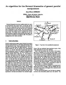
2. The description of an atom’s location, relative to a neighboring atom, in terms of the local internal coordinates for the bond that joins them. It should be clear that these two points define a recursive discrete integration problem on the internal coordinates. The first point is trivially solvable (simply specify the cartesian coordinates of the anchor atom). We proceed next to define the mathematical characterization of the second point. In order to describe the location of an atom relative to its neighbors, we define a coordinate system, or frame, attached to each atom, following the Denavit-Hartenberg (DH) method. In the DH local frames method, there is a local coordinate frame attached to every atom A i (see figure 1). The idea is to express the cartesian coordinates of atom Ai with respect to the coordinate frame attached to atom Ai−1 ; this will serve as the definition of our recursion step in the integration procedure outlined above, and obviously this conversion will involve bond parameters (i.e. angles and bond length). Once we have such a coordinate-frame conversion, we can propagate it towards the anchor atom A0 , for which we know its exact position. We will adopt the following convention to define local frames: frame Fi−1 = {Ai−1 , xi−1 , yi−1 , zi−1 }, where Ai−1 indicates the origin of the frame, and x, y, z the three orthogonal axes. Similarly, the local frame Fi attached to atom Ai is defined as Fi = {Ai , xi , yi , zi }. By convention axis zi lies along bond bi in the direction from Ai−1 to Ai ; this will simplify the math shortly. Axis xi−1 is chosen perpendicular to both zi−1 and zi (so that the bond angle αi can be defined around it) and can be obtained by their cross-product as in x i = zi−1 × zi . Finally, to complete a coordinate frame, yi is perpendicular to both xi and zi and can be obtained by their cross-product yi = xi × zi (in that order) to define a right-handed coordinate system. Keep in mind that this construction is only theoretical and does not actually need to be performed in a program; its sole purpose is to obtain a mathematical formula for the conversion, as will be shown. As depicted in Figure 1, the distance between atom Ai−1 and atom Ai , the bond length for bond bi , is denoted by di . The angle between zi−1 and zi , the bond angle, is denoted by αi−1 . Finally, the dihedral angle on bond bi is denoted by θi . The formal definition of the dihedral angle θi is the angle between the plane defined by atoms Ai−2 , Ai−1 and Ai and the plane defined by atoms Ai−1 , Ai and Ai+1 . Intuitively, θi defines the torsion of bonds bi−1 and bi+1 around bond bi . For the purpose of deriving one coordinate frame conversion, assume P is an arbitrary point in space, with coordinates (x, y, z) in frame Fi . We want to express these coordinates with respect to frame Fi−1 (to obtain our recursion formula). Then, (x0 , y 0 , z 0 , 1)t = Ri · (x, y, z, 1)t where (x0 , y 0 , z 0 ) are the coordinates of P with respect to frame Fi−1 , and Ri is the matrix that transforms frame Fi−1 to frame Fi . During the following discussion, you may want to keep inspecting figure 1 to validate the results (this may require several reads of this section). To obtain the above frame conversion, one approach is to apply succesive transformations to F i−1 until it coincides with Fi (the reader should convice him/herself that this is equivalent to obtaining the transformations that convert the coordinates of P from Fi to Fi−1 ; try creating some simple examples, by choosing simple P ’s, and following the conversion of coordinates for this point). First we need to remove the displacement between the origins of the frames, and then we need to align the frames, 4

Figure 1: Local frames Fi−1 and Fi attached to atoms Ai−1 and Ai , respectively. so that their axes coincide. To remove the displacement between the origins of the frames, one needs to translate frame Fi−1 along zi by the distance between the two frame origins, di . This translation can be expressed by the following matrix in homogeneous coordinates (recall that in homogeneous coordinates, translation, which is not a linear transformation, can be composed with other linear transformations by simple matrix multiplication):

1 0  Tzi (di ) =  0 0 

0 1 0 0

0 0 1 0

0 0   di  1 

(1)

After removing the displacement, one needs to align the two frames to make their axes coincide. Axis xi−1 does not coincide with axis xi due to the dihedral angle θi between them. Axis zi−1 does not coincide with axis zi due to the bond angle αi−1 between them. We first align xi−1 with xi , and then align zi−1 with zi . To align xi−1 with xi , one needs to perform a rotation by the dihedral angle θi around axis zi . This rotation is given by the following matrix:

cos(θi ) − sin(θi )  sin(θ ) cos(θi )  i Rzi (θi ) =   0 0 0 0 

0 0 1 0

0 0   0 1 

(2)

To align zi−1 with zi , one can perform the rotation by bond angle αi−1 around axis xi . This rotation is given by the following matrix: 5

1 0 0 0 cos(α ) − sin(α ) i−1 i−1 Rxi (αi−1 ) =   0 sin(αi−1 ) cos(αi−1 ) 0 0 0 

0 0   0 1 

(3)

Note that the order of rotations is important. One cannot perform the rotation of frame F i−1 by αi−1 first 0 and then the dihedral rotation, because a rotation by αi−1 changes the axis xi−1 to xi−1 . The value for the dihedral θi is defined with respect to xi−1 and xi , not xi−1 0 and xi . To do the rotation by the dihedral 0 second, you would need to update the definition of θi with respect to xi−1 since the axis xi−1 changed. This is not convenient since for every transformation you would need to recompute the dihedral angle; this is why a rotation by the bond angle first and the dihedral angle second is necessary. Now we can finally transform Fi−1 to Fi by combining the above matrices as follows: Ri = Rxi (αi−1 ) · Rzi (θi ) · Tzi (di ) where:

cos(θi ) − sin(θi ) 0 0 sin(θ ) cos(α ) cos(θ ) cos(α ) − sin(α ) − sin(α )d   i i−1 i i−1 i−1 i−1 i   Ri =   sin(θi ) sin(αi−1 ) cos(θi ) sin(αi−1 ) cos(αi−1 ) cos(αi−1 )di  0 0 0 1 



(4)

This formula provides all we need to integrate the atom coordinates from any starting point. As we said before, a generic step in the integration is to get the cartesian coordinates (x, y, z) of any atom A i with respect to frame Fi−1 as follows: (x, y, z, 1)t = Ri · (0, 0, 0, 1)t Recall that the coordinates of atom Ai in its own frame Fi are (0, 0, 0) since we defined each local frame as resting on the atom centers, so the origin of frame Fi is the atom Ai . When using internal coordinates, the position of atom A0 (the anchor atom) is the only one known, so every other atom’s cartesian coordinates can be obtained by chaining matrices R i . Since the local coordinates of atom Ai in its own frame are (0, 0, 0) (each local frame is attached to the center of an atom), its coordinates (x, y, z) with respect to the frame attached to the anchor atom are computed as follows: (x, y, z, 1)t = R1 · R2 · . . . · Ri · (0, 0, 0, 1)t Thus, for any value of i, we can retrieve Ai ’s position in terms of A0 and all the bond parameters between them (encoded in all the matrices). The only thing left to specify to globally place our protein is its orientation. One can allow for rotations or translations of the local frame attached to the anchor atom with respect to some global frame. Rotations of the anchor atom with respect to a global frame cause a rigid rotation of the entire polypeptide chain. To do so, one can define the rotation frame as the Euler matrix defined by the Euler angles of the local frame of the anchor atom to the global frame. 6

There are many conventions to define the Euler matrix. One of them, the X −Y −Z convention, defines the Euler matrix as the product of three rotation matrices: rotation around z by angle α; rotation around y by the angle β; rotation around x by the angle γ. In the X-Y-Z convention, the order is as follows: E = Rz (α) · Ry (β) · Rx (γ) This definition yields as the Euler matrix the one below: cos(α) cos(β) cos(α) sin(β) sin(γ) − sin(α) cos(γ) cos(α) sin(β) cos(γ) + sin(α) sin(γ)  sin(α) cos(β) sin(α) sin(β) sin(γ) + cos(α) cos(γ) sin(α) sin(β) cos(γ) − cos(α)sin(γ) E=   − sin(β) cos(β) sin(γ) cos(β) cos(γ) 0 0 0 

0 0   0 (5) 1 

Propagation of the rotation by the Euler matrix to the entire polypeptide chain can be done as follows: (x, y, z, 1)t = E · R1 · R2 · . . . · Ri · (x0 , y0 , z0 , 1)t Remember that all the protein’s internal coordinates (bond angles, bond lengths and dihedral angles) are encoded in the Ri matrices, so this formula provides the conversion between internal and cartesian coordinates we set out to find. For more information on the original application of Denavit-Hartenberg local frames to robotic mechanisms, see [1]. [1] J. Craig. Introduction to robotics: manipulation and control. Addison-Wesley, 2 edition, 1989.

7