An Algorithm of Speaker Clustering Based on ... - Semantic Scholar

348

JOURNAL OF MULTIMEDIA, VOL. 9, NO. 3, MARCH 2014

An Algorithm of Speaker Clustering Based on Model Distance Wei Li*, Qian-Hua He, Yan-Xiong Li, and Ji-chen Yang South China University of Technology School of Electronic and Information Engineering, Guangzhou, China *Corresponding author, Email: [email protected]

Abstract—An algorithm based on Model Distance (MD) for spectral speaker clustering is proposed to deal with the shortcoming of general spectral clustering algorithm in describing the distribution of signal source. First, an Universal Background Model (UBM) is created with a large quantity of independent speakers; Then, Gaussian Mixture Model (GMM) is trained from the UBM for every speech segment; At last, the probability distance between the GMM of every speech segment is used to build affinity matrix, and speaker spectral clustering is done on the affinity matrix. Experimental results based on news and conference data sets show that an average of 6.38% improvements in F measure is obtained in comparison with algorithm based on the feature vector distance. In addition, the proposed algorithm is 11.72 times faster. Index Terms—Spectral Clustering; Speech Signal Processing; Speaker Clustering; Audio Event; Model Distance

I.

INTRODUCTION

With the development of the streaming technology, the breakthrough in broadband transmission bottleneck and the increasing amount of media information, audio-video document (for example meeting audio-video, TV and movie audio-video, talk speech and broadcast audio), which is one of main media contents, is rapidly increasing [1-4]. How to organize, browse and retrieve the audio document effectively has been one urgent problem in media retrieval fields for researchers. Speaker clustering is an effective tool that can alleviate the amount of speech document management tasks [5-6]. Speaker clustering can group similar audio utterance together and attribute it to the same speaker in audio document by some distance measure and clustering scheme in the unsupervised condition [7]. Spectral clustering has been used in speaker clustering in recent years and has been proved to have better effect than hierarchical clustering [8-9]. It is because hierarchical clustering is a greedy search method, which can produce suboptimal solution and it has high computation complexity, however, spectral clustering can obtain a global optimal solution and its computation complexity is relatively lower. Spectral clustering is an algorithm based on graph theory [10-11], which translates clustering problem into multi way partitioning problem without direction graph. There are many concrete realization algorithms for it, for example, PF, SM, SLH, © 2014 ACADEMY PUBLISHER doi:10.4304/jmm.9.3.348-355

NJW, MS and so on [12], thereinto, NJW is one of the most widely used algorithms, spectral clustering that is used in this paper is on the base of NJW [13]. The main steps of speaker clustering using spectral clustering is as following: 1). Calculate the distance of two speech segments feature vector frame by frame, then calculate the similarity of the two speech segments by Gaussian kernel function based on the distance. 2). Construct affinity matrix of spectral clustering based on similarity. 3). Construct Laplace matrix by using affinity matrix, then decompose feature, construct feature vector space by using feature vector corresponding to the former k eigenvalues. 4). Cluster for all the feature vector of speech samples center the feature vector in the space using k-means and some classic clustering algorithms to realize speaker clustering. Affinity matrix of this clustering algorithm is constructed by feature vector distance of every speech segments. Speaker clustering takes into account the differences of the spatial distribution of source. The essence of speaker clustering based on feature vector distance is using the distance of samples to measure the similarity of every kinds, which is not enough to describe the differences of spatial distribution of source. And feature vector only can depict some characters of speech from the point of the single feature, which contains not only semantic content information but also speaker information and semantic content information is more than speaker information, so it is not enough to judge speaker similarity only using the distance of two speech segments [14]. In order to overcome the above mentioned problems of speaker clustering based on feature distance, a speaker clustering algorithm that is using model distance to construct affinity matrix is presented in this paper. It employs every speech segment for clustering according to MAP (Maximum A Posteriori), obtains GMM (Gaussian Mixture Model) of every speech segment for clustering adaptively, then constructs affinity matrix of spectral clustering by calculating probability distance based on a finite observation sequence model. GMM-UBM (Gaussian Mixture Model - Universal Background Model) is used in this paper can describe the speakers’ differences from the point of statistics adequately, GMM-


349

UBM can produce more precise model expression under the condition of a small voice training set, which has better robustness [15-16]. Probability distance based on a finite observation sequence model in this paper considers not only the models differences but also samples, and it can overcome the shortcoming of model description that is not accurate enough under the condition of the relative short length of speech segment. At last, experimental results based on many different experimental data sets show that an average improvements of 6.38% in F measure is obtained in comparison with traditional algorithm. In addition, the proposed algorithm is 11.72 times faster. II.

Speaker clustering based on model distance, which is presented in this paper mainly modifies the construction of the affinity matrix. It employs every speech segment for clustering according to MAP, and obtains UBM of every speech segment for clustering adaptively, then constructs affinity matrix of spectral clustering by calculating probability distance based on a finite observation sequence model, to cluster speakers for speech segments. A. Introduction of Speaker Spectral Clustering based on Feature Distance Most of the current speaker spectral clustering methods use feature distances between frames of speech segments to construct affinity matrix. The algorithm of speaker spectral clustering based on feature distance is as follows [8]: 1). Supposing S  S1 , S 2 , , Sn stands for speech



sample for clustering, n stands for the number of speech segments of speech samples. Si and S j stand for the ith and j-th speech segment, respectively, Ci  [ ]Ni D and

C j  [ ]N j  D

stand for their feature vector,

respectively, where N i and N j is speech number, respectively and D is feature dimension, obtaining distance matrix E   N  N of two speech segments i

j

by calculating Euclidean distance between Ci and C j frame by frame. 2). Calculate the minimum value row _ min Ni of every row in E and the minimum value col _ min N j in E in order, obtain the distance d ss (Si , S j ) of two speech segments by calculating the average value of the minimum value of row and column:  Ni 1     row _ min i  N i    1  i  0  d ss ( Si , S j )   N 1  2  j    col _ min N  j  j    j  0   

© 2014 ACADEMY PUBLISHER

 d ss 2  Si , S j    Aij  exp     2 ij2  

(1)

(2)

where the calculation formula of scale function  ij is as follows:



 ij   var  dss  Si ,    var d ss  , S j  where 



(3)

is a coefficient of preset, var stands for

calculating the variance, d ss  Si ,  

ALGORITHM INTRODUCTION



3). Use formula (3) to calculate every element in affinity matrix A, A  Rnn

stands for the

distance between speech segment Si and either speech segment except Si . 4). Calculate Laplace matrix L, L  D1 2 AD1 2 , where D is diagonal matrix and D (i, i)is the sum of every element in affinity matrix A. 5). Calculate the former k largest eigenvalues of Laplace matrix L and corresponding eigenvector  1 , 2 ,  k , construct matrix V  [ 1 , 2 ,  k ] , where i is column vector, V  Rnk and k is gotten by the method of eigen gap [8]. 6). Normalize the row vector of matrix V to obtain U  Rnk , U ij  Vij

V

2 ij

.

j

7). Let every row of matrix U be a point of R k space, for the points, use k-means or other methods to cluster to obtain k kinds. 8). If and only if the i-th row is divided into type j, speech segment Si will be divided into type j . From the above description, we can see that the algorithm mainly measures the similarity of every kinds by the distances of samples, however, speaker clustering mainly considers the differences of the spatial distribution of source. Feature vector only portrays some characters of speech from the point of single feature, comparatively speaking, it is more unilateral. It also calculates the feature vector distances of every speech segments, whose calculation is too huge. B. Speaker Clustering based on Model Distance The primary differences between the proposed algorithm and traditional algorithm is the calculation of affinity matrix, the proposed algorithm employs every speech segment for clustering according to MAP, obtains GMM of every speech segment for clustering adaptively, then constructs affinity matrix of spectral clustering by calculating probability distance based on finite observation sequence model. There are three advantages of the proposed algorithm: 1). The probabilistic distance calculates the similarity of every GMM-UBM which is using model based on finite observation sequence can describe the differences of the spatial distribution of source. It can not only

350


measure the similarity of two models but also join the different information of speech sequence. 2). GMM-UBM can describe the differences between speakers from the point of statistics and it can generate more sophisticated model description under a less speech training set, which has better robustness [15-16]. 3). The proposed algorithm’s computation is appreciably lower than speaker spectral clustering. The calculation method of affinity matrix based on GMM-UBM-MAP model distance, which is as follows: 1). Use plenty of speech of different speakers to train a UBM off-line. 2). Supposing S  S1 , S 2 , , Sn stands for speech





sample for clustering, Si and S j stand for the i-th and j-th speech segment, respectively. Make every speech segment for clustering to be adaptive using UBM according to MAP in turn, and obtain GMM G  G1 , G2 , , Gn of speech segment for clustering by





revising mean vector. 3). The probabilistic distance calculates the similarity which use a model based on finite observation sequence. The probabilistic distance of Gi for G j based on finite observation sequence is [17]:





1 D(Gi , G j )  log P  O j Gi   log P O j G j  (4)  Tj 

where Gi and G j is GMM of speech sequences



Oi  o1i , o2i , o3i ,

, oTi i



and



O j  o1j , o2j , o3j ,

, oTjj



adaptively, respectively, Ti and T j are the frames of O i and O j , respectively. Probabilistic distance formula (4) is asymmetrical, the definition of symmetric probabilistic distance formula is: Ds  Gi , G j  

1  D  Gi , G j   D  G j , Gi   2

(5)

4). The probabilistic distance which is a model between every GMM acts as the distance d ss (Si , S j ) of every speech segment, d ss (Si , S j )  Ds  Gi , G j 

(6)

5). Use formula (6) to calculate the every element of affinity matrix A.  d ss 2  Si , S j    Aij  exp     2 ij2  

(7)

where the calculation formula of scaling function  ij is:



 ij   var  dss  Si ,    var d ss  , S j 




(8)

where  is a constant coefficient, var stands for variance, d ss  Si ,   represents for the distance of speech segment

Si and any speech sample except Si . C. Algorithm Computation Complexity The differences between the proposed algorithm and speaker spectral clustering algorithm based on feature distance is the method of calculation affinity matrix A. Supposing the two algorithms employ the same feature, the differences of their computation is mainly in the distance computation between every speech segment. We analyze the computational complexities of two distance measures by taking the computation of distance between two speech segments as an example. Supposing feature matrix of two speech segments S1 and S 2 are C1  [ ]N1 D and C2  [ ]N2 D , respectively, where N1 and N 2 are the frame number of every speech segment, and D is feature dimension. According to formula (1) to calculate feature distance of two speech segments, calculation Euclidean distance of two feature vectors C1 and C2 frame by frame firstly. The Euclidean distance between i-th frame of C1 and j-th frame of C2 is: eij 

D

 (C d 1

i,d 1

 C2j , d )2

(9)

According to formula (9), the Euclidean distance computation of i-th frame of C1 and j-th frame of C2 is D times scalar subtraction, D-1 times scalar addition, D times scalar multiplication, and one time scalar evolution. The Euclidean distance matrix computation between C1 and C2 needs N1  N2 times Euclidean distance between frame and frame, that is D  N1  N2 times scalar subtraction, (D-1)  N1  N2 times scalar addition, D  N1  N2 times scalar multiplication, and N1  N2 times scalar evolution. Then, according to formula (1), under the premise of Euclidean distance formula E, it also need N1  N2  1 times scalar addition, three times scalar division, and N1  N 2 times taking the minimum value to calculate feature distance of two speech segments. In summary, the computation feature distance of two speech segments in formula (1) needs D  N1  N2 times scalar subtraction, (D-1)  N1  N2  N1  N2  1 times scalar addition, N1  N2 times evolution, D  N1  N2 times scalar multiplication, three times scalar division, and N1  N 2 times taking the minimum value。 D stands for feature dimension, i stands for the frame number of speech segment, and Gaussian mixture number is 16, the computation of GMM for a speech for clustering by using MAP adaptively is 16  i  D times scalar subtraction, i  D  32i  16D  16 times scalar addition, 17i  D  32D  18i times scalar multiplication, i  D  17i  16D  16 times scalar division and i times taking power of e. If the frame number of two speech is


40


20

0 0

10 20 30 40 T he appearance times of every speaker(T imes)

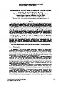
Figure 1. The speaker frequency distribution statistics in XWLB speech

2.5

EXPERIMENTAL RESULTS AND ANALYSIS

A. Experimental Data and Set Up Refer to the data types of speech diarization (SD) evaluating, Xin Wen Lian Bo (XWLB) and meeting speech are used to evaluate the proposed algorithm. These two speech data are very typical data in current speaker analysis and have different characters. It can get a more comprehensive evaluation for spectral clustering algorithm based on model distance by employing them as test datas. All the above mentioned data is sampled at 16KHz, 16bits, saved as mono channel wav format. There are seven speech segments of XWLB totally, the length of which varies from 1656s to 1803s, the number of speakers varies from 10 to 18, the rein to, the frequency of occurrence of anchorman, anchorwoman, male recording and female recording are higher, however, the other speakers, for example, interviewee and reporter only appear once or twice and the time length is too short. XWLB represents the inhomogeneous typical case of speaker speech sample distribution. There are eight meeting speech segments, the length of which vary from 1505s to 2420s, the number of speakers in which vary

30

10

2

Frequency(%)

III.

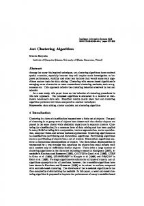
from 4 to 10. There are little differences for the guest speaking times in the meeting speech, because anchorperson is in charge of the conference, the speaking times is relatively more, some questioners only appear once or twice, but the number of questioners is usually from 2 to 5, so the appearance times of every speaker in meetings are relatively more balanced and speaking time length for each time is longer. Meeting speech represents the more homogeneous scene of speaker speech sample. Figure 1 and 2 represent the speaker frequency distribution statistics in XWLB speech and meeting speech. Taking the leftmost column in Figure 1 for example, it means that the frequency of speakers who appear only once in XWLB is 42%. From figure 1 and 2, it is observed that the number of speakers who appears only once is more and distribution of speech sample is very uneven in XWLB, however, the number of occurrences of every speaker in meeting speech is more balance.

Frequency(%)

N1 and N 2 respectively, the computation of GMM for the two speech segments is 16  ( N1  N2 )  D times scalar subtraction, ( N1  N2 )  D  32( N1  N2 )  16D  16 times scalar addition, 17( N1  N2 )  D  32D  18( N1  N2 ) times scalar multiplication, times scalar ( N1  N2 )  D  17( N1  N2 )  16D  16 division and N1  N 2 times taking power of e. According to formula (4) and (5), the computation between two models based on finite observation sequence model of probability distance is 16(N1  N2 )  D times scalar subtraction, 16(N1  N2 )  D times scalar addition, times scalar 16(N1  N2 )  D  16(N1  N2 )  16D multiplication, 16(N1  N2 )  D  16(N1  N2 )  1 times scalar division, 16 times evolution, 16(N1  N2 ) times taking power of e, and N1  N 2 times taking log. In summary, the computation model distance of two speech segments is 16  17( N1  N2 )  D times scalar subtraction, 17( N1  N2 )  D  32( N1  N2 )  16D  16 times scalar addition, times scalar 33( N1  N2 )  D  34( N1  N2 )  48D multiplication, 17( N1  N2 )  D  33( N1  N2 )  16D  17 times scalar division, 16 times evolution and 17( N1  N2 ) times taking power of e and N1  N 2 times taking log. A speech segment usually has over 2s length, according to sample rate 16KHz, frame length 32ms and frame shift 16ms to calculate, a speech segment contains 124 frames at least, so the computation of feature vector distance of every speech segment is more than computation of model distance of every speech segment.

351

1.5

1

0.5

0 0

20 40 60 T he appearance times of every speaker(T imes)

80

Figure 2. The speaker frequency distribution statistics in meeting speech

Table I gives the primary information of experimental data, which contains speaker times (ns), the longest length of speech segment (lmax), the total speech segments (#ss), the segment number with the length of speech varying from 0 to 10s (#ss0-10), the segment number with the length of speech varying from 10s to 20s (#ss10-20), the segment number with the length of speech varying from

352


20s to 30s (#ss20-30), the segment number with the length of speech above 30s (#ss30) and the average length of every segment speech (lavg). TABLE I. Audio sorts XWLB Meet

MAIN INFORMATION OF TEST DATA (MEETING: MEET) ns 93 52

lmax 303 453

#ss 500 273

#ss0-

#ss10-

#ss20-

10

20

30

127 93

225 26

71 26

#ss30 77 128

lavg (S) 24.43 55.11

The experimental platform used is Intel(R)Core(TM)2 Duo CPU P8400 2.26GHz, 3 GB RAM, Windows XP operation system, program software Visual Studio 2008. Speaker segment is used for every speech file by the manual annotation, then every speech segment is framed and extracted 24 dimensions MFCC feature, the time length of which is 32ms and the frame length is 16ms. After extracting feature, affinity matrix is constructed based in feature vector distance and spectral clustering method of construction affinity matrix based on model distance is clustered, respectively. The experimental results of the two methods are compared finally. The UBM of clustering using model distance clustering method is trained by 16 GMMs offline and the training speech is 300 different speakers who are from 863 speech libraries and the time length of every speaker is 3s.The mixture number of GMM of every speech segment for clustering adaptively is 16. B. Evaluation Index Evaluation index of speaker clustering are mainly average cluster purity (ACP) and average speaker purity (ASP) [18]. N s stands for the total number of speaker, N c stands for the total sort number, nij stands for all speech frames spoken by j-th speaker in i-th sort, the definition of ACP is as follows: Nc

Nc

ACP   max (nij ) i 1

Ns

 n

j1, N s 

ij

(10)

ij

(11)

i 1 j 1

The definition of ASP is as follows: Ns

ASP   max (nij ) j 1

i1, Nc 

Nc

Ns

 n i 1 j 1

Finally, F is used as the overall performance evaluation index and the definition is as follows: F

2  ACP  ASP ACP  ASP

(12)

C. Experimental Result and Analysisi Table II and Table III give speaker confusion based on model distance spectral clustering in a audio file of XWLB and meeting speech, respectively, the column stands for real speakers, the row stands for speaker speech clustered. There is only a speaker in a sort, the ACP of the sort is 100%, the more people in a sort, the less ACP. When all the speech of a speaker is clustered in a sort, the ASP of the speaker is 100%, when the speech


of a speaker is clustered into more sorts, the ASP of speaker less. The most ideal clustering effect is that the sort is the same as speaker number, every speaker is only assigned to a sort and there is only a speaker in a sort. It is observed that: speaker G and I are both clustered 0-th sort, speaker H, J and speaker A whose lengths are very short are all clustered 7-th sort, speaker E and B are clustered 2-nd sort, speaker F and C are clustered 3-rd sort. From table II, we can see that the speech lengths of speaker E, F, G, H, I, J are relatively shorter, and it is easy to make mistake in the construction of GMM, so it is ease confusion in the clustering. From table III, it can be seen that speaker B, D and speaker A whose lengths are shorter are clustered into 1st sort, confusion is more serious. It is found that speaker B and D are both male by using human’s ear to hear their corresponding audio, and the speed and pronunciation of speaking are both very similar, it is difficult to distinguish. The traditional algorithm and the proposed algorithm are respectively test, and the results are listed in table IV and V. The tables give the relevant information of speech length len, speaker number #sp, clustering sort number #cl, average speech processing time every second. From table IV, we can know that, ACP, ASP and F using the proposed algorithm to cluster for XWLB speech are 86.25%, 90.62% and 88.08%, respectively, the average cost time of speech whose length is one second is 0.55s, compared with the traditional algorithm, F improves 4.46%, runspeed is 11.72 times faster than latter. From table V, it can be seen that, ACP, ASP and F using the proposed algorithm to cluster for meeting speech are 86.47%, 93.19% and 89.31%, respectively, and the average cost time of speech whose length is one second is 0.38s, compared with the traditional algorithm, F improves 8.29%, runspeed is 12.13 times faster than latter. Whether using XWLB speech or meeting speech for clustering speech, comparison with tradition algorithm, F of the proposed algorithm can be improved a little and F can be improved more for processing meeting speech. The primary reason is that GMM-UBM is built firstly in the proposed algorithm, the accuracy of the building model is relatively lower for short lengths, which influence the clustering affect, comparatively speaking, the tradition algorithm has less influence than the proposed algorithm for the segment length. The number of short speech segment in XWLB speech is more than that in meeting speech, so the improvement of the proposed algorithm is more obvious than traditional algorithm for processing meeting speech. It can be seen that the differences between clustering sort and real speaker number are obvious from table IV and V, the primay reason is that spectral clustering is a unsupervise clustering method, and the clustering number is decised by eigen gap [11], the method of determining the number of clusters has some differences with reality. In order not to reduce F and reduce comoputation complex as much as possible, how the longest speech sample length influences the proposed algorithm is test in


TABLE II.

SPEAKER CONFUSIONS USING BROADCAST NEWS AUDIO FILE TO EVALUATE THE MODEL DISTANCE BASED SPECTRAL CLUSTERING METHOD (UNIT: S) (SORT: SOR) Speaker A B C D E F G H I J

TABLE III.

353

Sort 0

Sort 1

Sort 2

Sort 3

Sort 4

157.76 170

Sort 5

Sort 6

Sort 7 1.34

Sort 8 101.16

7.82 239.05 834.48

195.50

14.59 16.30 18.39 19.80 14.25 12.58

SPEAKER CONFUSIONS USING CONFERENCE AUDIO FILE TO EVALUATE THE MODEL DISTANCE BASED SPECTRAL CLUSTERING METHOD (UNIT : S) (SORT: SOR ) Speaker A B C D E TABLE IV. alg TRA ALG

The Pro Alg

TABLE V.

Sort 0 0.99

Sort 1 10.99 355.73

Sort 2

Sort 3 1.52

Sort 4 62.03

Sort 5 186.97

Sort 6 1.04

322.22 434.88 473.64 OADCAST SPEECH (ALGORITHM :ALG) (TRADITIONAL: TRA) (PROPOSED : PRO)

audio file 1 2 3 4 5 6 7 mean 1 2 3 4 5 6 7 mean

Len (s) 1683 1656 1803 1784 1790 1724 1776

#sp 12 14 10 16 13 10 18

#cl 8 9 9 6 9 8 5

1683 1656 1803 1784 1790 1724 1776

12 14 10 16 13 10 18

7 8 9 7 8 7 8

ACP (%) 80.04 81.60 92.20 81.91 89.44 89.56 78.86 84.80 82.90 81.18 94.17 84.05 88.57 91.57 81.29 86.25

ASP (%) 84.69 61.93 84.74 95.11 84.78 82.81 88.09 83.16 83.82 99.18 94.94 98.38 84.53 78.13 95.37 90.62

F (%) 82.30 70.42 88.31 88.02 87.05 86.05 83.22 83.62 83.36 89.28 94.55 90.65 86.50 84.32 87.92 88.08

Time (s) 6.72 6.36 5.81 5.63 6.13 6.21 6.71 6.22 0.58 0.57 0.48 0.49 0.54 0.59 0.61 0.55

TEST RESULT OF CONFERENCE SPEECH (ALGORITHM :ALG) (TRANDITIONAL: TRA) (PROPOSED : PRO)

alg TRA ALG

The Pro Alg

audio file 1 2 3 4 5 6 7 8 mean 1 2 3 4 5 6 7 8 mean

Len (s) 1688 1505 1667 1603 2128 1850 2420 2184

#sp 7 7 4 4 10 5 6 9

#cl 10 7 7 6 7 9 6 9

1688 1505 1667 1603 2128 1850 2420 2184

7 7 4 4 10 5 6 9

8 9 5 11 8 7 9 8

this paper, which can provide the experimental basis for compromise between F and computation complex, when the length of single speech sample for clustering is more than ns, the speech segment with ns length is intercepted


ACP (%) 66.66 64.59 98.44 82.29 67.17 73.47 70.40 80.68 75.46 92.11 92.64 99.61 91.75 86.75 80.09 70.14 78.66 86.47

ASP (%) 82.73 84.59 92.61 87.18 89.70 87.99 88.27 91.42 88.06 94.29 92.10 99.85 87.89 80.11 95.86 97.92 97.49 93.19

F (%) 73.83 73.25 95.44 84.66 76.82 80.08 78.33 85.72 81.02 93.19 92.37 99.73 89.78 83.30 87.27 81.74 87.07 89.31

Time (s) 4.66 4.09 3.76 3.62 5.48 5.02 5.28 4.95 4.61 0.39 0.35 0.42 0.28 0.43 0.42 0.33 0.39 0.38

to be as representative for clustering, but in calculation clustering result, the length of speech sample segment is according to the intercepting length.

354


ACP, ASP, F and processing time of every second speech averagely of 5s, 10s, 20s, 30s speech intercepted segment of XWLB and meeting speech are respectively given in table VI and VII. TABLE VI.

CLUSTERING RESULT OF NEWS BROADCAST SPEECH INTERCEPTED N SECONDS

N (s) 5 10 20 30

ACP (%) 83.24 85.25 85.73 85.92

TABLE VII. N (s) 5 10 20 30

ASP (%) 85.92 86.07 88.75 89.84

F (%) 84.56 85.66 87.21 87.84

Time (s) 0.28 0.38 0.46 0.52

CLUSTERING RESULT OF MEETING SPEECH INTERCEPTED N SECONDS

ACP (%) 75.25 76.35 79.47 85.23

ASP (%) 80.87 88.307 90.932 92.59

F (%) 77.96 81.89 84.82 88.76

Time (s) 0.19 0.22 0.26 0.30

From table VI and VII, we can see that, when the length of the interception of speech is more, F bigger, and when the length reaches 30s, the clustering result is the same as all test speech segments joined .According to the result, when we calculate the clustering for long speech segments, we can intercept 30s speech as representative to cluster, which not only save runtime but also have little influence on the results. From table VI and VII, we also can see that, the results improve little when the length of interception speech is 30s and 20s for dealing with XWLB speech, however, for dealing with meeting speech, F of 30s can improve more than 20s, the primary reason is that the rate of the length over than 30s in meeting speech is more than that in XWLB speech. IV.

CONCLUSIONS

This paper presents an algorithm of speaker spectral clustering based on model distance. The proposed algorithm uses GMM-UBM-MAP to obtain adaptively model of every speech segment in the construction of the affinity matrix, the model, which is using adaptive model of every speech segment based on finite observation sequence, for the probability distance between the GMM of every speech segment is used to build affinity matrix, then the speakers are clustered. compared with the algorithm based on feature vector distance, F can improve 6.38%, the computation speed is about 11.72 times as much as the latter, which means that the proposed algorithm is more effective for speaker clustering. Finally, the length of test speech sample affecting clustering result is discussed in this paper, the length of test speech sample is longer, the clustering effect better, when the length reaches 30s, the clustering result is the same as all test speech segments joined . ACKNOWLEDGMENT This work is supported by the National Nature Science Foundation of China (61301300), China Postdoctoral Science Foundation (2013M531850) and the Fundamental Research Funds for the Central Universities, SCUT, China (2013ZM0097).


REFERENCES [1] Y. Yang, F. P. Nie, D Xu, et al. “A multimedia retrieval framework based on semi-supervised ranking and relevance feedback,” IEEE Transactions on Pattern Analysis and Machine Intelligence, 2012, Vol. 34, pp. 723–742. [2] Jitao Sang, Changsheng Xu. “Faceted Subtopic Retrieval: Exploiting the Topic Hierarchy via a Multi-modal Framework,” Journal of Multimedia, 2012, Vol. 7, pp. 9-20. [3] Qing Li, Hon Chung Mak, Jianmin Zhao, Xinzhong Zhu. “OXML: an Object XML Database Supporting Rich Media Indexing and Retrieval,” Journal of Multimedia, 2011, Vol. 6, pp. 115-121. [4] Ji-chen Yang, Lei-an Liu, Qing-wei Qin, Min Zhang. “Audio Event Change Detection and Clustering in Movies,” Journal of Multimedia, 2013, Vol. 8, pp. 113-120. [5] H. Tang, S. Chu, et al. “Partially supervised speaker clustering,” IEEE Transactions on Pattern Analysis and Machine Intelligence, 2012, Vol. 34, pp. 959-971. [6] Y. -X. Li, Y. Wu, Q-H. He, “Feature mean distance based speaker clustering for short speech segments,” Journal of Electronics & Information Technology, 2012, Vol. 34, pp. 1404-1407. (In Chinese) [7] W. Jeon, C. Ma, D. Macho, “An utterance comparison model for speaker clustering using factor analysis,” IEEE International Conference on Acoustics, Speech and Signal Processing, 2011, pp. 4528-4531 [8] Iso K. “Speaker clustering using vector quantization and spectral clustering,” IEEE International Conference on Acoustics, Speech and Signal Processing. Dallas, 2010: 4986-4989. [9] H Z Ning, M Liu, H Tang, et al. “A spectral clustering approach to speaker diarization,” IEEE Proceedings of the 9th International Conference on Spoken Language Processing. Pittsburgh, 2006: 2178-2181 [10] J Z Cao, P Chen, Y Zheng, et al. “A Max-Flow-Based similarity measure for spectral clustering,” ETRI Journal, 2013, 35(2): 311-320. [11] Jia J H, Xiao X, Liu B X, et al. “Bagging-based spectral clustering ensemble selection,” Pattern Recognition Letters, 2011, 32(10): 1456-1467. [12] Xiao-yan Cai, Guan-zhong Dai, Li-bin Yang. “Survey on Spectral Clustering Algorithms,” Computer Science, 2008, 35(17): 14-18. [13] A. Y. Ng, M. I. Jordan, Y. Weiss, “On spectral clustering: analysis and an algorithm, Advances in Neural Information Processing Systems,” Cambridge: MIT Press, 2002: 849856 [14] Dong-xing Xu, “Text-independent speaker verification based on GMM and high-level information,” Hefei: Department of Electronic Science and Technology, University of Science and Technology of China, 2009. (In Chinese) [15] X Wang, Q Yin, P Guo. “Text-independent Speaker Identification Using Fisher Discrimination Dictionary Learning Method,” IEEE International Conference on Computational Intelligence and Security. Beijing:, 2012: 435-438. [16] Y H Chao, W H Tsai, H M Wang. Improving “GMMUBM speaker verification using discriminative feedback adaptation,” Computer Speech and Language, 2009, 23(3): 376–388. [17] Qian-Hua He, Yi-qin Lu, Gang Wei, “A new approach for HMM training,” ACRA Electronica SINICA, 2000, 28(9): 56-58. (In Chinese)


[18] X, Zhang, J. Gao, P. Lu, et al. “A novel speaker clustering algorithm via supervised affinity propagation,” IEEE International Conference on Acoustics, Speech and Signal Processing, Las Vegas:, 2008: 4369-4372.

355

years in 4 periods. From 2007.11 to 2008.10, he worked with University of Washington in Seattle as a visiting scholar.

Wei Li was born in Tonghua, Jilin province China in November, 1979. She received the B.S. Degree in applied electronic technology from JiLin University, Changchun, Jilin province, China, in 2002, and the M. S. Degree in measurement and testing technologies and instruments from JiLin University, Changchun, Jilin province, China, in 2006. From August 2006 to July 2008, she worked as a teaching assistant associate with the Department of Electronic and Information at Zhuhai College of Jilin University. Now she is pursuing her Ph. in telecommuncation and information system at South China University of Technology. Her current interest is speech/audio signal processing.

Yan-xiong Li was born in Jiahe, Hunan province, China, in Aug. 1980. He received the B. S. Degree and the M. S. Degree both in Electronic Engineering from Hunan Normal University(HNU) in 2003 and 2006, respectively, and the Ph. D degree in communication and Information System from South China University of Technology in 2009. From 2 September 2008 to 1 September 2009, he worked as a research associate with the Department of Computer Science at the City University of Hong Kong. From 23 March 2010 to present, he has been working as a lecturer with the School of Electronic and Information Engineering at South China University of Technology. His current research interests include speech/audio signal processing, pattern recognition. He has two research grants from the National Natural Science Foundation of China and from the Natural Science Foundation of Guangdong Province, China.

Qian-hua He was born in Shaodong, Hunan province, China, in Feb. 1965. He received the B. S. Degree in physics from Hunan Normal University in 1987, the M. S. Degree in medical instrument engineering from Xi'an Jiaotong University in 1990, and the Ph. D degree in communication engineering from South China University of Technology, in 1993. Since 1993, he has been at the Institute of Radio and Autocontrol of South China University of Technology. His research interests include speech recognition, speaker recognition and its security, optimal algorithm design, such as genetic algorithm and neural networks, embedded system design. From 1994 to 2001, he worked with the department of computer science, City University of Hong Kong for about 3

Ji-chen Yang was born in Jieshou, Anhui province China in June, 1980. He received the B.Eng. degree in electronic and information engineering from Guangdong University of Petrochemical Technology (GUPT), Maoming, Guangdong province, China, in 2004, he received the M. Eng. Degree in system engineering from Guangdong University of Technology, Guangzhou (GUTC), Guangdong, China, in 2007.he received the Ph.D. in Telecommuncation and information system from South China University of Technology (SCUT), Guangzhou, Guangdong, China, in 2010. Now he is a post doc. researcher in South China University of Technology. His current interest is movie audio signal processing.
