AN ALGORITHMIC APPROACH TO INFERRING CROSS-ONTOLOGY ...

Serdica J. Computing 6 (2012), 309–332

AN ALGORITHMIC APPROACH TO INFERRING CROSS-ONTOLOGY LINKS WHILE MAPPING ANATOMICAL ONTOLOGIES Peter Petrov, Milko Krachounov, Ernest A. A. van Ophuizen, Dimitar Vassilev

Abstract. Automated and semi-automated mapping and the subsequently merging of two (or more) anatomical ontologies can be achieved by (at least) two direct procedures. The first concerns syntactic matching between the terms of the two ontologies; in this paper, we call this direct matching (DM). It relies on identities between the terms of the two input ontologies in order to establish crossontology links between them. The second involves consulting one or more external knowledge sources and utilizing the information available in them, thus providing additional information as to how terms (concepts) from the two input ontologies are related/linked to each other. Each of the two ontologies is aligned to an external knowledge source and links representing synonymy, is-a parent-child, and part-of parent-child relations, are drawn between the ontology and the knowledge source. These links are then run through a set of simple logical rules in order to come up with cross-ontology links between the two input ontologies. This method is known as semantic matching. It proves useful ACM Computing Classification System (1998): J.3. Key words: ontology, anatomical ontology, ontology mapping, anatomical ontology mapping, probability, scoring, external knowledge source, algorithm, graph, directed acyclic graph.

310

P. Petrov, M. Krachounov, E. A. A. van Ophuizen, D. Vassilev and reasonably accurate; in this paper, we call it the source matching predictions (SMP) procedure. Not all cross-ontology links that semantically (i.e., from a biological/anatomical standpoint) exist between the two input ontologies will be discovered by either DM or SMP. To improve the discovery of cross-ontology links we propose a novel algorithmic procedure which involves a probability-like scoring scheme. This procedure is called the child matching predictions (CMP) procedure. Describing the DM, SMP, CMP procedures, and particularly the CMP procedure in formal terms is the main goal of this paper.

1. Introduction. Ontologies are formal models for knowledge representation and knowledge modeling. A widely adopted definition is that “an ontology is an explicit and formal specification of a conceptualization of a domain of interest” [5]. Two main aspects are highlighted by this definition – first, that the specification is formal, which implies that automatic reasoning can be performed on it, and secondly, that it is practically oriented towards a particular domain of interest. Another informal definition can be found in [6]; it states that “an ontology grasps the entities which exist within a given portion of the world at a given level of generality, it includes a taxonomy of the types of entities and relations that exist in that portion of the world seen from within a given perspective”. This definition focuses again on two aspects – first, that an ontology models only a portion of the world, which implies its specifici, and second, that an ontology has a formal structure (called taxonomy) that includes the entities that exist (in the portion of the world that is being modeled) and the relations which exist among them. Important problems in the research area which deals with ontologies are those of ontology integration or mediation [1]. The two terms, integration and mediation, are pretty much synonymous but the latter is preferred for the purposes of this paper as it has already been adopted by most authors. Ontology mediation concerns integrating ontologies that model identical or similar domains but which have different origin. The importance of the ontology mediation problem comes from the fact that ontologies are designed and developed by different parties (research groups, business organizations) and it cannot be expected that these parties will ever agree on using a common ontology even though the domain being modeled is similar or even identical. As noted in [1], two principal types of ontology mediation exist – ontology mapping and ontology merging. Mapping is about establishing links/bridges between two (or more) ontologies without altering them. The result of the mapping process of several input ontologies is, in principle, not an ontology but a

An Algorithmic Approach to Inferring Cross-Ontology Links . . .

311

set of semantic links/bridges/correspondences between the ontologies. That result doesn’t replace the original ontologies, but supplements them and is stored separately of the input ontologies. Merging is about taking two ontologies and generating a single ontology from them that unifies/unites the knowledge contained in the input ontologies. The result of the merging process is a single output ontology that could be used as a replacement of the two input ontologies. Another important concept related to ontology mediation is ontology alignment – the process of automatic or semi-automatic discovery of links between ontologies [1], as opposed to manual discovery of these links. In particular, special attention should be paid to the cases of alignment of heterogeneous ontologies based on different conceptualizations of the same problem domain [3, 4]. For the purposes of this work, it is assumed that two given ontologies can be aligned to each other, but also to some external knowledge sources (which may or may not be ontologies themselves). For solving the general ontology mediation problem, various efforts have been made in the last decade that usually produce theoretical models, which then serve as a basis for practical program or framework implementations. We list here only the most prominent or popular ones: (i) ontology mapping – MAFRA [8], RDTF [9], and IF-Map [10], (ii) ontology merging – PROMPT [11], and OntoMerge [12], (iii) ontology alignment – Anchor-PROMPT [13], GLUE [14], QOM [15, 16], S-Match [17, 18]. Excellent surveys of the ontology mediation research field can be found in [1], [2], and [19]. In this work, we deal with an ontology mapping and merging problem within a very specific, practical context. This is the problem of mapping and merging anatomical ontologies of two or more different species/organisms. The problem is important for at least two different reasons. First, the ability to perform cross-species automated text searches (text mining) in scientific literature can produce valuable results. It enables a researcher designing experiments in a particular model organism (e.g., mouse) to draw upon earlier findings in a different model organism (e.g., zebrafish), without needing to be an expert on both systems. Anatomical ontologies of many different species are nowadays publicly available, but no intelligent tools exist that are able to perform intelligent cross-species text searches (or text mining) in these ontologies or in various text sources that contain anatomical information about the different species (e.g., mouse, rat, chicken, zebrafish). What is needed is the ability to perform searches that don’t rely solely on simple text identities between term names in order to report these terms as synonyms (e.g., head(mouse) = head(rat)), but which would be intelligent enough to detect cross-species synonyms whose

312

P. Petrov, M. Krachounov, E. A. A. van Ophuizen, D. Vassilev

textual representations have nothing in common (for instance fin(zebrafish) = wing(chicken) = foreleg(mouse, rat)). Here the equality sign denotes an anatomical similarity (roughly speaking) or homology (strictly speaking) between anatomical terms of different species. It is apparent that to achieve these goals, the different species-specific anatomical ontologies need to be mapped onto each other and (in the ideal case) ultimately merged into a single output anatomical super-ontology. Second, having two species-specific ontologies mapped onto each other and possibly merged into a common super-ontology would enable tools which currently work with the anatomical ontology of one species to support more than the species-specific ontology which they were originally designed for. That is, solving the ontology mapping problem could extend the capabilities of existing tools and could make them more intelligent and more powerful. Once the anatomical super-ontology is there, existing tools could be ported (with some effort) to the super-ontology which resulted from merging the two input species-specific anatomical ontologies. This would turn those tools from single-species aware to multi-species aware. Due to the very specific nature of the problem, a very specific approach is presented here which does not have any claims to generality but rather to specificity and biological (in particular anatomical) adequacy of the results. The general methods listed above usually try to map, merge or align ontologies modeling the same or similar domains of interest. In this work, the domains modeled by the input ontologies are rather similar when viewed from one angle (as they are both anatomical domains) but rather distinct when viewed from another angle (as they represent the anatomies of two different species which may or may not be closely related from an evolutionary standpoint). Due to the specific nature of the problem, it is possible to interrogate specific biomedical knowledge sources (like UMLS1 [22], FMA2 [23]) and to utilize their knowledge which inherently imparts certain intelligence to the software program (AnatOM [7]) that implements the algorithmic procedures presented in this paper. However, the specificity of the problem does not prevent AnatOM from also interrogating general-purpose knowledge sources (like WordNet3 [20, 21]). Talking to such general-purpose knowledge sources proves very useful as they provide valuable additional insights to inferring links between the ontologies which are subject to mapping and ultimately to merging. 1

http://www.nlm.nih.gov/research/umls/ (2012) http://sig.biostr.washington.edu/projects/fm/ (2012) 3 http://wordnet.princeton.edu/ (2012) 2


313

2. An overview of the problem domain. Anatomy is a branch of biology and medicine that studies the structures of the living things (organisms, species). Three main branches of anatomy exist – (i) human anatomy, (ii) animal anatomy (zootomy), (iii) plant anatomy (phytotomy). This work deals with (ii) even though some of its ideas and methods are applicable also to (i) and (iii). Anatomy can also be divided into (a) macroscopic anatomy which studies structures that can be observed even with the naked human eye, and (b) microscopic anatomy which studies structures that the naked human eye cannot observe. Of these two, this work deals mostly with (a). The algorithmic procedures presented in this paper take two anatomical ontologies as input (e.g., the adult mouse anatomical ontology and the ontology of the zebrafish anatomy and development) and map them onto each other. The two input ontologies are encoded in OBO [24, 25] which is a formal language for representing ontologies (like OWL [27] and RDF-Schema [28]). The OBO ontology language is used mainly in the biomedical sciences and in bioinformatics; its computer representation is a plain text file format which is also known as OBO. This plain text file format is easily readable by both humans and computer programs; it allows for describing the terms/concepts from the domain that is modeled together with the relations that exist among these terms/concepts. For the purposes of this work, the ontologies originally encoded in OBO are first translated to mathematical (graph theoretical) forms, and the procedures presented below work on these mathematical forms. The algorithmic procedures themselves are also described in mathematical terms and not in pseudo-code or in some practical programming language.

3. Formal definition of the problem. 3.1. The two input ontologies. Two input ontologies are given in the form of OBO files. For the purposes of this work each of these ontologies is viewed as a directed acyclic graph (DAG) [7] together with an edge-coloring function. The two ontologies used as examples here are the mouse O1 = OM and the zebrafish O2 = OZ anatomical ontologies but the method presented below is applicable to other couples of species-specific anatomical ontologies, e.g., (mouse, rat), (mouse, chicken), (chicken, zebrafish). In the text below the following notations are used. O1 : DAG1 = (V1 , E1 ); F1 : E1 → C = {c1 , c2 , . . . , cn} O2 : DAG2 = (V2 , E2 ); F2 : E2 → C = {c1 , c2 , . . . , cn}

314


Here O1 and O2 are the two input ontologies each of which is considered as composed of a directed acyclic graph DAGk and an edge-coloring function Fk. Also here, C = {c1 , c2 , . . . , cn} is the set of colors, F1 and F2 are two coloring functions which are associated with the two directed acyclic graphs DAG1 and DAG2 . Each color represents one inner-ontology relation of subsumption of certain kind (inverse generalization, i.e., specialization; inverse aggregation, i.e., membership; etc.). The relations is-a (specialization) and part-of (membership) are the two typical examples of such inner-ontology relations defined within OBO ontologies and within anatomical OBO ontologies in particular. Therefore, for the purposes of this work, it can be assumed that n = 2, c1 = is-a, c2 = part-of. In the notation introduced above, V1 is the set of anatomical terms/concepts in the mouse anatomical ontology and V2 is the set of anatomical terms/concepts in the zebrafish anatomical ontology. V1 = {v11 , v12 , . . . , v1n1 }, |V1 | = n1 V2 = {v21 , v22 , . . . , v2n2 }, |V2 | = n2 . Each ontology term vij has two components which are both strings (idij , nameij ), where idij is the identifier (the id) of the term/concept vij , and nameij is the textual name of the term/concept vij . In general, the term ids are unique within the ontology bounds but are not globally unique. Theoretically, if two different ontologies are given, it is possible that there exist two terms, one term from the first ontology and the other one from the second ontology, which are distinct but whose ids are equal. Practically, in our case, all mouse term ids begin with the string “MA” and all zebrafish term ids begin with the string “ZFA” so it is impossible to have two terms (one from mouse, one from zebrafish) sharing the same term id. In the two ontologies O1 and O2 each term t = (id, name) may optionally also have a set of alternative names or what is called inner-ontology synonyms. Within the first ontology, the edge e1 = (v1i, v1j ) ∈ E1 if and only if the term v1i is a child of the term v1j in the graph DAG1 . The same applies to the second ontology, i.e., the edge e2 = (v2i, v2j ) ∈ E2 if and only if the term v2i is a child of the term v2j in the graph DAG2 . Here, “child” is a generalized concept meaning either an is-a or a part-of child. Throughout this text we refer to O1 and O2 as the two input ontologies. 3.2. The three external knowledge sources. Also given are several large external knowledge sources (biomedical or general-purpose ontologies) which contain anatomical terms and relations (is-a, part-of, others) among those terms. In particular, three concrete external knowledge sources are used for the purposes of this work. These are T1 = UMLS, T2 = FMA, T3 = WordNet. Although


315

questionable if these knowledge sources are indeed ontologies (in the strict sense), they are viewed and used as such for the purposes of this work. Formally put, each of these knowledge sources Ts (s = 1, 2, 3) contains the following information. • Set of terms Ms = {ts1 , ts2 , . . . , tsms }, where tsk = (idsk, namesk) and idsk is the identifier (the id) of the term/concept tsk, namesk is the textual name of the term/concept tsk, ms is the count of terms in the knowledge source Ts. It should be noted at this stage that: i) it is sometimes possible that tsi 6= tsj but namesi = namesj (same names, different ids); ii) it is sometimes possible that tsi 6= tsj but idsi = idsj (same ids, different names); iii) in this notation, the ids and the names are strings and the equalities (or inequalities) above express identity (or lack of identity) between the strings involved. • Relations of subsumption Each knowledge source Ts also defines (at least) the following two relations: ′ is_a RTs = RTs ⊆ Ms × Ms ′′

part_of

RTs = RTs ⊆ Ms × Ms These two are the is-a and part-of relations (again) but in the way they are defined by the knowledge source Ts. Additional relations are usually also defined within Ts but the is-a and part-of are of greatest interest for the purposes of this work. 3.3. The problem goal. Using the available knowledge sources T1 = UMLS, T2 = FMA, T3 = WordNet and the is-a and part-of relations which they define between their own terms, a set of reliable (authentic, trustworthy) semantic relations between the terms of the two input ontologies O1 and O2 has to be found. These semantic relations should be biologically (anatomically, evolutionary) justified and should be of one of the following types. Type 1. Synonyms – R1 = Rsyn – terms with similar or identical meaning are called synonyms. Type 2. Hypernyms – R1 = Rhyper – generalization – a hypernym is a term whose semantic range includes that of another term (its hyponym) – Fig. 1. Type 3. Hyponyms – R1 = Rhypo – specialization – a hyponym is a term whose semantic range is included within that of another term (its hypernym) – Fig. 1. Type 4. Holonym – R1 = Rholo – aggregation – term X is a holonym of term Y, if Ys are parts of (members of) X – Fig. 2.

316


Fig. 1. An is-a parent-child relation

Fig. 2. A part-of parent-child relation

Type 5. Meronym – R1 = Rmero – membership – term Y is a meronym of term X, if Ys are parts of (members of) X – Fig. 2. The goal here is to establishSrelations of the types just described (from 1 to 5) such that Ri ⊆ (V1 × V2 ) (V2 × V1 ), for i = 1, 2, 3, 4, 5 and such that these relations are authentic (make sense, i.e., are biologically valid, i.e., are evolutionary justified) based on the knowledge that is available in the external knowledge sources T1 = UMLS, T2 = FMA, T3 = WordNet. Of greatest interest is establishing the relations of Type 1 (the synonymy relations or R1 = Rsyn as these allow for mapping the two input ontologies O1 and O2 onto each other, and ultimately for merging them into one common output super-ontology which we denote as Osuper .

4. The algorithmic solution. In this paper an integrated algorithmic approach to solving the problem is proposed. The method consists of three main stages which we briefly outline here. • Stage 1: Generate the thesauri Within this stage from the mouse ontology O1 its thesaurus T h1 is built, and analogically from the zebrafish ontology O2 its thesaurus T h2 is built. • Stage 2: Align the two input ontologies to the three knowledge sources Within this stage each of the two input ontologies O1 and O2 is aligned to each of the three knowledge sources available T1 = UMLS, T2 = FMA, T3 = WordNet. In fact, within this stage not the ontologies themselves, but the thesauri T h1 and T h2 that have been generated from them, are aligned to the three external knowledge sources. Still, we usually say that the two input ontologies are aligned to the three external knowledge sources. • Stage 3: Infer cross-ontology synonymy links/relations, and crossontology parent-child (is-a/part-of) links/relations. This stage consists of three phases which we outline here.


317

• Phase 3.1: Synonymy links are drawn for syntactic or direct matches between the terms from O1 and O2 . This is what we denote as the direct matching (DM) procedure. • Phase 3.2: Using the results from Stage 2 (the alignments performed there) and a set of simple logical rules, cross-ontology synonyms are predicted. This is what we call the source matching predictions (SMP) procedure. • Phase 3.3: For pairs of terms t1 ∈ V1 and t2 ∈ V2 for which no synonymy relation has been discovered so far, the relations hereto predicted between t1 ’s and t2 ’s children are used, in order to infer additional predictions about how t1 and t2 are related. That’s what we call the child matching predictions (CMP) procedure. This procedure infers new predictions about relations which seem to exist between t1 and t2 even though these relations don’t directly originate from the knowledge contained in the three external knowledge sources. In the next subsections, the three stages which were only briefly outlined here, are described in more details. 4.1. Stage 1 – Generating the thesauri. The thesauri T h1 of O1 and T h2 of O2 are simple dictionary-like tabular structures. For the id of any term t ∈ V1 , the thesaurus T h1 maintains a list T h1[t.id] that contains the primary name and all the alternative names (if any) of the term t ∈ V1 with identifier id. In the same way, for the id of any term t ∈ V2 , the thesaurus T h2 maintains a list T h2 [t.id] containing the primary name and the alternative names (if any) of the term t ∈ V2 with identifier id. The lists T hi[t.id] (i = 1, 2) are simple lists of strings. Their members are all the names (as defined by the input ontologies) of the term t with the given identifier id. Building the thesauri from the two input ontologies is a fairl straightforward process. 4.2. Stage 2 – Aligning the input ontologies to the knowledge sources. In this stage each of the two input ontologies (each of the two thesauri) is aligned to the three external knowledge sources. Below is described how the ontology O1 (i.e., its thesaurus T h1 ) gets aligned to the external knowledge source T1 . The other alignments are performed analogically. Phase 2.1: For each term id k ∈ O1 do → get the list L = T h1 [k] from the pre-built thesaurus T h1 . Phase 2.2: For each term name s ∈ L do → get from T1 all distinct ids (T1 ’s term ids) which correspond to the term name s, i.e., get RS1 = {(tI .id) | tI ∈ T1 and tI .name = s} Step 2.2.1: For each id from RS1 do → get from T1 RS2 = {(tII .id, tII .name) | tII ∈ T1 and tII .id = tI .id}

318


Having performed this step, the result is that the synonyms of s (as they are defined by T1 ) are now known. These are also denoted as the T1 -synonyms of s – technically this is the set RS2∗ = {tII .id | tII ∈ T1 and tII .id = tI .id} composed of the first components of the ordered couples contained in RS2 . Step 2.2.2: For each id from RS1 do → get from T1 the set is_a

RS3 = {(tIII .id) | tIII ∈ T1 and ((tIII , tI ) ∈ RT1

or (tIII , tI )

part_of

)} ∈ RT1 Having performed this step, the result is that the followings sets are now known • the meronyms of s as defined by T1 . These are also called the T1 meronyms of s – technically this is the set part_of RS3,1 = {tIII .id | (tIII , tI ) ∈ RT1 } • the hyponyms of s as defined by T1 . These are also called the T1 hyponyms of s – technically this is the set is_a RS3,2 = {tIII .id | (tIII , tI ) ∈ RT1 } Is should be noted that RS3,1 ∪ RS3,2 = RS3 , RS3,1 ∩ RS3,2 = ∅. Step 2.2.3: For each id from RS1 do → get from T1 the set is_a

RS4 = {(tIV .id) | tIV ∈ T1 and ((tI , tIV ) ∈ RT1

or (tI , tIV )

part_of

∈ RT1 )} Having performed this step, the result is that the following sets are now known • the holonyms of s as defined by T1 . These are also called the T1 holonyms of s – technically this is the set part_of } RS4,1 = {tIV .id | (tI , tIV ) ∈ RT1 • the hypernyms of s as defined by T1 . These are also called the T1 hypernyms of s – technically this is the set is_a RS4,2 = {tIV .id | (tI , tIV ) ∈ RT1 } Again, it should be noted that RS4,1 ∪ RS4,2 = RS4 , RS4,1 ∩ RS4,2 = ∅. To summarize all this in plain words—the steps 2.2.1, 2.2.2, and 2.2.3 find in the external knowledge source T1 the following sets of T1 -terms: • Step 2.2.1—synonyms of the original ontology-defined term s with id k; • Step 2.2.2—meronyms and hyponyms of the original ontology term s with id k; • Step 2.2.3—holonyms and hypernyms of the original ontology term s with id k;


319

These steps complete the process of aligning the input ontology O1 (i.e., its thesaurus T h1 ) to the external knowledge source T1 . Then, in an identical manner, O2 is aligned to T1 . Finally O1 and O2 are separately aligned to T2 and T3 (i.e., four more alignments are performed) by applying the exact same procedure as described here. 4.3. Stage 3 – Inferring cross-ontology synonymy and crossontology parent-child (is-a and part-of ) links/relations. In this stage three separate algorithmic procedures are applied, which are denoted as DM , SMP and CMP . They are described here in full details. Phase 3.1: Within this phase (called DM) textual/syntactical/direct matches/predictions for cross-ontology synonyms are found by checking for textual identities between the term names in the two ontologies. This procedure is straightforward, the algorithm just iterates through all terms t1 ∈ V1 and t2 ∈ V2 and tests if t1 .name = t2 .name. Whenever such matches are found, the terms t1 and t2 are marked as synonyms and it is noted (memorized) that this synonymy prediction comes from direct matching (DM). Here is a simple example: In O1 (the mouse anatomy ontology) there exists a term t1 = (id = “M A0000168′′ , name = “brain′′), while in O2 (the zebrafish anatomy ontology) there exists a term t2 = (id = “ZF A0000008′′ , name = “brain′′). So by doing the checks in this step, it is easily found that their names are identical (“brain”) and so these terms are marked as cross-ontology synonyms coming from DM. Phase 3.2: Within this phase (called SMP) more predictions are inferred for synonymy links and for parent-child links between the terms of the two input ontologies. As the two input ontologies have already been aligned to the external knowledge sources available, a set of logical rules is applied which results in inferring/predicting what is called source matching synonymy and source matching parent-child (is-a and part-of ) predictions. The rules applied in this phase are as follows. Rule A: If two terms tM ∈ O1 and tZ ∈ O2 have been detected as synonyms of the same term t ∈ Ti (by step 2.2.1) we mark tM and tZ as a predicted (by SMP) cross-ontology synonyms of each other. Rule B1: If tM ∈ O1 has been detected as synonym of t ∈ Ti (by 2.2.1) and if term tZ ∈ O2 has been detected as (is-a/part-of ) child of t (by 2.2.2), we mark tM as a predicted (by SMP) cross-ontology (is-a/part-of ) parent of tZ .

320


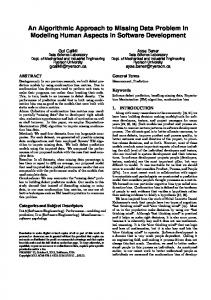
Rule B2: If tZ ∈ O2 has been detected as synonym of t ∈ Ti (by 2.2.1) and if term tM ∈ O1 has been detected as (is-a/part-of ) child of t (by 2.2.2), we mark tZ as a predicted (by SMP) cross-ontology (is-a/part-of ) parent of tM . Rule C1: If tM ∈ O1 has been detected as synonym of t ∈ Ti (by 2.2.1) and if term tZ ∈ O2 has been detected as (is-a/part-of ) parent of t (by 2.2.3), we mark tM as a predicted (by SMP) cross-ontology (is-a/part-of ) child of tZ . Rule C2: If tZ ∈ O2 has been detected as synonym of t ∈ Ti (by 2.2.1) and if term tM ∈ O1 has been detected as (is-a/part-of ) parent of t (by 2.2.3), we mark tZ as a predicted (by SMP) cross-ontology (is-a/part-of ) child of tM . By applying the above described rules, a set of cross-ontology relations (synonymy and parent-child) is drawn (established) between the nodes of DAG1 and DAG2 (i.e., between the terms of the two ontologies). These predicted links or relations are said to come from source matching inference (SMP) because the evidence of their existence originates from the information stored in the external knowledge sources that are used. It should also be noted that for the so-inferred parent-child links, the information whether these are is-a or part-of links is also stored. This completes the description of the SMP procedure. Before proceeding with the formal description of phase 3.3 (the so-called child matching predictions (CMP) procedure), here is a short recap itulation of what has been done so far. Several new notations and definitions are introduced here which are going to help us in describing the CMP procedure (the last phase 3.3 of stage 3). The two original (input) graphs DAG1 and DAG2 defined above are available. The cross-ontology links which have been inferred so far (in 3.1 – DM and in 3.2 – SMP ) are also available. Now, the two original graphs together with the links established by DM and SMP can be thought of as one single graph G = (V, E), where V = V1 ∪ V2 and E = SIO ∪ SDM ∪ SSMP , where • SIO is the set of all inner-ontology links in DAG1 and DAG2 ; • SDM is the set of all links inferred in phase 3.1, i.e., by direct matching (DM); • SSMP is the set of all links inferred in phase 3.2, i.e., by the source matching predictions (SMP) procedure. The properties of each of these types of links are summarized in the table on Fig. 3. • The IO links are the original links from the two input ontologies. These are always parent-child links and are colored/labeled either with is-a or with part-of . These are unidirectional links as the parent-child relations are not symmetrical.

An Algorithmic Approach to Inferring Cross-Ontology Links . . . Link Type Synonymy or Parent-child Color/Label IO Links Only parent-child Either is-a or part-of DM Links Only synonymy No color/label SMP Parent-child Links Parent-child Either is-a or part-of SMP Synonymy Links Synonymy No color/label

321

Symmetry Unidirectional Bidirectional Unidirectional Bidirectional

Fig. 3. Links and link types

• The DM links are cross-ontology links which by their definition (phase 3.1) are always synonymy links and as such they are colored neither with is-a nor with part-of . As the synonymy is a symmetrical relation, these are bidirectional links, i.e., we may think of each DM link (t1 , t2 ) or t1 ←→ t2 as a pair of two links t1 → t2 and t1 ← t2 . • The SMP links are either parent-child links (steps 2.2.2 and 2.2.3 of phase 2.2) or synonymy links (step 2.2.1 of phase 2.2). As with the IO and DM links: the parent-child SMP links are colored either with is-a or with part-of and are unidirectional; the synonymy SMP links have no color/label and are bidirectional. All SMP links are cross-ontology ones by their definition (steps 2.2.1, 2.2.2, 2.2.3 from phase 2.2 and rules A, B1, B2, C1, C2 from phase 3.2). All this having been said, the single graph G (as defined above), which has been produced from DAG1 and DAG2 by the DM and SMP procedures, can now be considered. Phase 3.3: The description of the CMP procedure is what follows next. This description is intermixed with several definitions which allow us to arrive at one final number that we call final/aggregated CMP score of the aggregated CMP link that gets drawn between any two nodes v1 ∈ E1 and v2 ∈ E2 that are involved in certain patterns of connectivity within the graph G. Definition 1. Constant I – reliability score of an inner-ontology (IO) link. Typically I = 1 but this value could be varied/adjusted if needed. Definition 2. Constant D – reliability score of a direct matching (DM) link. Typically D = 1 but this value could be varied/adjusted. Definition 3. Constants f (UMLS), f (FMA), f (WordNet) – reliability scores of the three available knowledge sources. We require that: 0