1
An algorithmic game-theory approach for coarse-grain prediction of RNA 3D structure Alexis Lamiable1,2 , Franck Quessette1 , Sandrine Vial1 , Dominique Barth1 , Alain Denise2,3,4,∗
Abstract—We present a new approach for the prediction of the coarse-grain 3D structure of RNA molecules. We model a molecule as being made of helices and junctions. Those junctions are classified into topological families that determine their preferred 3D shapes. All the parts of the molecule are then allowed to establish long-distance contacts that induce a threedimensional folding of the molecule. An algorithm relying on game-theory is proposed to discover such long-distance contacts that allow the molecule to reach a Nash equilibrium. As reported by our experiments, this approach allows one to predict the global shape of large molecules of several hundreds of nucleotides that are out of reach of the state-of-the-art methods.
the modules, by classifying the junctions into topological families; we then put them together to build the global shape of the molecule. Finally, this shape is improved by discovering potential interactions between separate parts of the secondary structure. We compare two approaches to this step: a global optimization algorithm, and a novel game theory approach that favors local, egoistical choices instead of searching for a global optimum.
Index Terms—RNA, tertiary structure prediction, coarse-grain structure prediction, game theory
A. Workflow overview
I. I NTRODUCTION
R
NA molecules fold into complex three-dimensional structures, and knowing that structure is of great help to determine biological function. RNA structure is hierarchical, with a secondary structure made of canonical Watson-Crick base-pairs forming first, followed by a tertiary structure involving several other interaction types [25]. Prediction of the secondary structure from one or several sequences is well studied and provides good results, especially when sequence alignments are available. Ab initio single sequence approaches include Mfold [27] and RNAfold [7], that use dynamic programming to optimize a free-energy function. Other approaches, like CONTRAfold [4], do not rely on an energy function but on a stochastic model with learned parameters. Most of the approaches are restricted to secondary structures without pseudoknots, but some can predict pseudoknots, at a higher complexity cost. Comprehensive reviews of various approaches can be found in [5] and [13]. Automatic prediction of the tertiary structure, and of the three-dimensional (3D) shape of RNA molecules is still a very difficult task. The most efficient ab initio prediction software packages, iFoldRNA [24], FARNA [3], NAST [9] and MC-Fold/MC-Sym [21], can handle molecules of about one hundred nucleotides. In this paper, we take advantage of the modular and hierarchical nature of RNA structures to predict the general shape of 3D structures of larger molecules. We present a coarse-grain, step-by-step approach in which we consider a molecule to be made of helices and junction between helices (modules). We first determine the shape of 1: 2: 3: 4: *:
PRiSM, Univ. de Versailles-St-Quentin-en-Yvelines / CNRS, France. LRI, Univ. Paris-Sud / CNRS, Orsay, France. IGM, Univ. Paris-Sud / CNRS, Orsay, France. INRIA Saclay, France. Corresponding author:
[email protected]
II. M ATERIALS AND METHODS The general workflow for our prediction is as follows: 1) build a coarse-grain representation of the secondary structure without pseudoknots, called a skeleton graph, representing helices and junctions between helices; 2) classify the junctions into 3D topological families (local 3D shapes); 3) assemble all those local shapes together, to obtain an initial embedding of the skeleton graph in 3D without tertiary interactions; 4) try to predict (coarse-grain) new interactions between the distant nodes of the skeleton graph. These longdistance interactions can take part in the tertiary structure and are used to obtain the final shape of the molecule. The idea behind that last step is that the initial embedding represents an ideal shape where each node is locally satisfied, but that it neglects the possibility for the nodes to establish interactions with other nodes that might provide more stability. These interactions induce a folding of the molecule away from its initial embedding, into a more stable form. We explored two ways to predict long-distance interactions: by maximization of a global payoff function, and by searching a stable configuration (possibly a Nash equilibrium) in a game where each node tries to maximize its own payoff function. We now expand on all the steps of that general workflow, and introduce a payoff function suitable for both approaches. B. Models 1) Skeleton graph: we use a coarse-grain representation of the structure of the molecule, that we call a skeleton graph (see Fig. 1). Each helix or junction between helices is represented by a node. Nodes are linked by a secondary edge if the two corresponding helices or junctions are adjacent in the secondary structure, and by a long-distance edge if the
2
corresponding helices or junctions are modeled as being linked by long-distance interactions that contribute to the tertiary structure.
topological families. In this section, we briefly describe our classification methods, for each order of junction. In a previous paper [16], we have shown that three-way junctions can be automatically classified into three topological families, called A, B and C. These families, as shown in Fig. 3, are local, three-dimensional shapes, independent of the context of the molecule. From the secondary structure of a three-way junction, without information about the context of the molecule, we predict the correct family 64% of the time, and this performance is noticeably improved by using several homologous secondary structures. Family A
Fig. 1. Skeleton graph superimposed on the secondary structure of 1NBS (bacterial RNase P). An example of a tertiary interaction is shown on the secondary structure as a dotted line, and the corresponding long-distance edge in the skeleton graph is shown as a thin line. Figure created with VARNA [2].
As we have just said, junctions are modeled as a node in the graph. However, for distance and angle computations, considering the position of the center of that node is too imprecise; we notably lose the intuitive idea of a stacking between two helices as a straight line. To solve that problem, we represent n-way junctions as a node with n handles to which the neighboring nodes can attach (see Fig.2). Those handles form a solid body during 3D transformations, and can be seen as points on the surface of a sphere that represents the junction.
Fig. 2. In the three-way junction pictured left, all helices seem equivalent, and no stacking is apparent. If we picture the junction as a sphere with three handles, and attach helices to the handles, the stacking becomes obvious.
We call a skeleton graph that contains no long-distance edge a secondary skeleton. In the rest of this paper, we do not consider pseudoknots in the secondary structures we start from, and consider that long-distance interactions include pseudoknots. Each node of the skeleton graph is associated with the set of corresponding nucleotides in the detailed structure. Moreover, each junction node of the skeleton is classified into a topological family, as described in the following section. 2) Classification of the junctions: our approach relies on the correct classification of RNA junctions (or multiloops) in
Fig. 3.
Family B
Family C
Families A, B and C of three-way junctions, as published in [18].
We have developed a similar method for classifying fourway junctions. Those junctions have been studied previously and classified into nine families [14]. Of these nine families, only three contain several instances in multiple molecules, families H, cH and cL. We only tried predicting those three well represented families. In order to avoid overfitting due to the low number of available four-way junction crystal structures, we did not apply any machine learning technique, and used only strand lengths criteria, by putting strands in three categories: short (≤ 3 nt), long (3 or 4 nt) or verylong (≥ 5 nt) (see Fig. 4). We now describe the “if-then-else” criteria we used: 1) if there are two short strands on opposite parts, for example (short-long-short-long) or (short-short-short-long), then we predict a stacking between the helices linked by those strands; 2) if we have a (short-long-short-long) configuration, with short being 2 or 3 nt, then we predict family cH; 3) if the two long strands are very long (more than 4 or 5 nt), we predict family cL; 4) if at least three strands are short, we predict family H; 5) in the case where all strands are short, we order them by transcription order, and predict a family H with stacking on the second and fourth strands); 6) if none of those rules apply, we do not give a prediction. Family H
Family cH
Family cL short
short
short short
long short
short
short
short
very long
long
Fig. 4. The three main families of four-way junctions. Single-strands are considered short if they include 3 nt or less, and long otherwise.
3
Using only those lengths criteria, we predict 44% of the four-way junctions studied in [14] in the correct family. We fail to predict 36% of the junctions in either family H, cH or cL, but this is a correct answer, since they do not belong in any of those families. Finally, we provide an incorrect prediction for 20% of the junctions. Since we use only very general criteria, and do not take the sequence into account, these are very promising results. The eventual availability of more four-way junctions in the databases will be useful for both confirmation of the validity of our criteria (particularly the fifth one) and the creation of classification criteria for the junctions that do not belong to families H, cH or cL. In our study, two-way junctions were considered more flexible than helices, but were not classified in topological families. Since angles between helices can vary greatly between different families (for example between a Kink-turn and a C-loop), introducing such a classification would be an interesting perspective. Preliminary work suggests that we can reliably distinguish between some two-way families, based on observations from [17]. Finally, junctions involving more than four helices represent less than 4% of all the junctions available in the crystal structure databases. While their shapes have been studied in [12], the observed “families” contain at most two different instances, which makes it impossible to study regularities and establish meaning classification criteria. Until more crystal structures of big RNA molecules are made available, we will leave higher order junctions unclassified. 3) Initial embedding: let S be a skeleton graph, and C be a classification of its junction nodes in families. We can embed S in 3D space by putting the first node n at a random position, and then recursively adding its neighbors, as illustrated in Fig. 5. This gives an initial “ideal” embedding where the helices adjacent to each junction j have exactly the desired angles according to C(j) and the desired length according to the base-pairs they represent. 1-way
helix
3-way
constraints in the graph. This induces a folding of the initial embedding to satisfy those constraints. We model this folding of the molecule with a spring-based graph drawing algorithm inspired from [11]. In this algorithm, the constraints are modeled by springs with various parameters and, by repeated small movements, an equilibrium between the forces exerced by the springs is reached. We use different spring parameters for different types of constraints. We have springs: • connecting a junction node with a helix node, modelling half-helices; • connecting a helix node with the center between the two neighboring junctions, modelling that helices tend to be straight, not bent; • connecting a junction node with its ideal position according to the classification of another junction it is connected to; • connecting any two nodes, modelling tertiary, longdistance interactions. 5) Payoff function: after reaching a stable shape when applying the spring algorithm, we define the cost of this embedding for a node as the sum of the absolute values of all the forces applied to that node. This cost represents how much the final shape deviates from the initial embedding. However, since we hope to discover long-distance interactions automatically, there must be an incentive for nodes to establish those interactions. Each long-distance interaction between two nodes reduces the costs of those nodes by a fixed amount, representing the contribution of that interaction to the stability of the molecule. The cost function for a node n is then: X X cost(n) = |force(s)| − I(e) (1) e∈LD(s) s∈springs(n) where springs(n) is the set of springs that apply to n, LD(n) the set of long distance interactions involving n, and I(e) the gain attributed to a single long-distance interaction. In our study, we considered I(e) to be a constant, independent of the nature of the interaction e. As it is more common to think about payoffs than costs in game theory, we then define the payoff of an embedding for a node as the maximum possible cost minus the cost of that node: payoff(n) = max(cost) − cost(n). (2)
Fig. 5. Creation of the initial embedding by adding successively the local 3D shapes of the components of the secondary structure. Each part should be seen as a three-dimensional shape, despite being shown in 2D here. Angles and distances in 3D are determined by the topological families of the junctions, and the lengths of the helices.
As we will see in section III-A, the initial embedding of a secondary skeleton can be very close to the real (coarse-grain) shape of a molecule, assuming the junctions were correctly classified. 4) Folding of the initial embedding: we can think of the initial embedding as the shape the molecule would have if it were void of long-distance tertiary interactions. Adding longdistance interaction means introducing additional distance
C. Discovery of long-distance interactions 1) Global optimization: in order to use the payoff function defined above to automatically find long-distance interactions, the first idea is to use a global optimization approach to maximize, for instance, the sum of the payoffs of all the nodes. We used a genetic algorithm [6], [8], where individuals represent possible sets of long-distance interactions. The algorithm we used is defined as follows: 1) Starting with a population of X individuals 2) Set aside the X/2 individuals with the best fitness 3) Create X/2 new individuals by crossing the ones from step 2
4
4) Add random changes to the individuals 5) Go to step 2 until the population is stable 6) Return the individual with the best fitness An individual is a set I of long-distance edges between nodes of the skeleton graph. However, in order to reduce the number of possibilities, we constrain the total nomber of longdistance edges to be lower than n (the number of nodes) by allowing each node to pick at most one interaction partner (see Fig. 6).
Algorithm 1: Linear reward-inaction [23] 1 2 3 4 5 6 7 8 9
2
while algorithm did not converge do foreach player i do actions[i] = select(Pi ) end payoffs = payoff function(actions); foreach player i do update vector(Pi , payoffs[i]) end end
1
Algorithm 2: Update of the probability vector after a player i Node Partner
1 ∅
2 4
3 1
4 1
4
3
played strategy action and gained payoff 1 2 3
Fig. 6. One possible individual in our population. In this example, node 1 makes no interaction, node 2 makes an interaction with node 4, and so on.
The fitness of an individual I is defined as the sum of the payoffs of all the nodes of the skeleton graph S after we have added all the long-distance edges of I to S and applied the folding algorithm defined in II-B4. 2) Game theory: it is well known that, for global optimization approaches to structure prediction, the optimal structure is not necessarily close to the real structure. This can be due to inaccuracies in the energy model, but also to the fact that, in vivo, molecules do not try to globally maximize their stabilities, but fold due to local contacts that are locally stable. This usually leads to a search among the structures that are close to a global optimum with regards to the energy function, hoping to find the real structure among them. In this paper, we study another approach by replacing global optimization with a local optimization, where each component of the molecule maximizes its own payoff function, egoistically. Reaching equilibria by means of a local, selfish optimization is the subject of game theory [26]. This leads us to model the folding problem as a game where each node of the skeleton graph is a player that tries to maximize its own payoff function. In this game, the players’ strategies to try to increase their payoffs is to establish one interaction with another node. Nash equilibria [19] are situations where no player can increase its payoff by changing its strategy by itself (but payoff can increase if two or more players change their strategies simultaneously). Being in a Nash equilibrium does not mean that players maximize their payoffs, but that they have nothing to gain by changing their stategies alone, and as such, Nash equilibria are stable situations. Finding them is one of the main goals in game theory. The problem of finding a Nash equilibrium is thought to be difficult in general [20]. We define our game as follows: the players are the nodes of the skeleton graph; each player can choose an interaction partner (ie. a node), or choose no partner; finally, the payoff function for each node is the function defined in equation (2) of Section II-B5. The set of all the players’ choices of strategies is similar to the individuals we defined for our evolutionary algorithm (Fig. 6).
4 5 6 7 8
c = number of strategies s with Pi [s] > 0 ; x = b × payoff × (1 − Pi [action]); Pi [action] = Pi [action] + x; foreach strategy s do if Pi [s] > 0 and s 6= action then Pi [s] = Pi [s] - x/c; end end
In our game, each of the n players has n possible strategies: finding a partner among the n − 1 other nodes, or no partner at all. Hence, there are nn possible combinations of strategies, which makes it impossible to compute the payoff matrix entirely. We treat the payoff function as a black box. This gives us a very general game where it seems difficult to compute a Nash equilibrium. Therefore, we use a reinforcement learning approach, in order to find an equilibrium by repeating the game many times. We implemented a linear reward-inaction algorithm given in [23] (Algorithm 1), where each player i keeps a probability vector Pi , where Pi [s] denotes its probability of picking strategy s (ie. choosing an interaction partner) when playing the game. The game is repeated and, at each step, the players pick their strategies, compute their payoffs, and then update their probability vectors to increase the likelihood of picking the same strategy again. The amount by which the probability is increased depends on the payoff that the player obtained, as described in Algorithm 2. In this algorithm, the parameter b slows the convergence down and it is shown in [23] that if b tends to zero and the algorithm converges, it converges to a Nash equilibrium. Algorithm 1 is not very practical, because the parameter b needs to be very small so that the algorithm does not converge to an incorrect solution, which leads to a very large number of iterations for all but the simplest games. Those iterations cannot be parallelized because the probability vectors need to be updated at each step, depending on the result of the previous iteration. We propose a modification of this algorithm that aims at greatly reducing the number of iterations needed to converge by increasing the cost of each iteration, in a way that allows parallelization to compensate for the added cost. Our
5
TABLE I M OLECULES STUDIED PDB Id
Name
1E8O 1MFQ 1NBS 2A64
Core of Alu Domain, Mammalian SRP S-Domain Complex of Human SRP Specificity Domain, Ribonuclease P RNA Bacterial Ribonuclease P RNA
TABLE II RMSD BETWEEN THE INITIAL EMBEDDING OF THE SKELETON GRAPHS AND THE EMBEDDINGS OBTAINED FROM CRYSTAL STRUCTURES . Nucleotides 49 127 155 417
modification is to replace line 3 in Algorithm 1 by a MonteCarlo method. Instead of drawing its strategy according to its probablity vector, each player performs X simulations of the game for each of its possible strategies, and picks the strategy that gave him the best average payoff. In those simulations, the player assumes that other players will follow their probability vector (which can be viewed as the frequency of their choices). This algorithm can be viewed as performing a best-response strategy [1] on a sampling of what the other players played before. This modified algorithm requires Xn2 calls to the payoff function, instead of one call for Algorithm 1. However, those calls are independent and can be parallelized. Using GPU cards, all the calls can be done simultaneously, even for large molecules, making one iteration of our algorithm as fast as one iteration of Algorithm 1. This algorithm is similar to the Sampled Fictitious Play (SFP) algorithm [15], with a different update rule. One notable difference is that, in SFP, the sample size is chosen when an iteration starts (and should increase at each step to avoid convergence wells), whereas in our algorithm, each player can choose its own sample size. By computing the standard deviation of the payoffs obtained for one strategy, one can adjust the sample size dynamically. III. R ESULTS AND DISCUSSION We report results of our approaches on a set of four molecules from the PDB, shown in Table I, and compare them to other known approaches. These molecules were chosen because they are representative of various sizes of RNA molecules, contain 3-way junctions, and because we have ˚ or good crystal structures for them (ie. with resolution 3.5 A better). Larger structures like subunits of the ribosome were considered, but the amount of large junctions that we cannot classify puts them out of our reach for the time being. Small structures without junctions are, too, outside the scope of this method. A. Accuracy of the initial embedding In order to verify whether the initial embedding of the molecules is close to their real shape, we computed the RMSD [10] between the initial embeddings of the skeleton graphs and embeddings computed from the crystal structures of the four molecules. The initial embeddings were computed by putting helices and junction nodes at the geometric center of all the atoms that they represent. In those initial embeddings, all the junctions were assumed to be predicted in the correct family. The results are given in Table II. In this table, the
PDB Id 1E8O 1MFQ 1NBS 2A64
Nodes
Nucleotides
RMSD
Junctions
7 19 21 37
49 127 155 417
3.53 6.10 10.29 21.18
3 3 4, 3 6, 4, 3, 3, 3
complexity of the molecules is measured both in terms of the number of nodes in the skeleton graph and of its composition in junctions. For example, molecule 1NBS contains 21 nodes, 1 three-way and 1 four-way junction. As we can see, the RMSD between the initial embedding and the real shape is relatively low and, as expected, grows with the complexity of the molecules. As we will see in ˚ the following subsection, obtaining a RMSD of about 10 A for a molecule of the complexity of 1NBS already is an improvement over what can be done with other programs. B. Comparison of global optimization and game theory TABLE III R ESULTS FOR GLOBAL OPTIMIZATION . Molecule Initial
˚ RMSD (A) Genetic
Real
1E8O C 1E8O A 1E8O B
3.53 5.89 7.86
3.48 6.00 8.17
3.80 4.66 7.08
1MFQ C 1MFQ A 1MFQ B
6.10 14.99 23.78
6.88 7.57 23.69
5.97 7.33 13.20
1NBS C 1NBS A 1NBS B
10.29 17.28 26.53
9.38 8.86 28.30
8.39 8.56 17.28
2A64 CAC 2A64 AAA 2A64 CCC
21.40 21.36 25.61
23.22 23.40 26.88
19.82 19.67 24.74
1) Results for global optimization: Table III shows the RMSD values between predicted structures and skeletons derived from the crystal structures, for four molecules and, for each molecule, several classifications of the junctions (see figure 3). The correct classification is shown in bold. For each molecule/classification pair, we computed the RMSD values for the initial embedding, the embedding resulting from the global optimization step do discover longdistance interactions, and the one obtained by providing the folding algorithm with the real tertiary interactions, as found in the PDB structures (“Real” column). This last value gives a lower bound to the RMSD values we can hope to obtain by predicting the long-distance interactions (even though it is still possible to obtain a lower RMSD by chance). As we can see in Table III, when the junctions are correctly predicted in the first place, the optimization step does not produce a significant change in RMSD. Introducing the real interactions only marginally improves the RMSD, which
6
proves that the initial embedding is good to begin with. However, when junctions are incorrectly predicted, sometimes, the optimization steps can correct the error. Finally, in the last molecule (2A64, RNase-P), we do not see any improvement in the RMSD, no matter what the initial classifications were. This is because, for that molecule, most of the error is due to the presence of a 6-way junction. Since we do not have a classification for that junction, it is represented as a regular hexagon.
Global:
Game:
TABLE IV R ESULTS FOR GAME THEORY.
Initial
˚ RMSD (A) Game
Real
1E8O C 1E8O A 1E8O B
3.53 5.89 7.86
3.98 5.42 7.94
3.80 4.66 7.08
1MFQ C 1MFQ A 1MFQ B
6.10 14.99 23.78
5.65 7.15 22.32
5.97 7.33 13.20
1NBS C 1NBS A 1NBS B
10.29 17.28 26.53
9.71 16.63 28.13
8.39 8.56 17.28
2A64 CAC 2A64 AAA 2A64 CCC
21.40 21.36 25.61
23.58 24.14 26.75
19.82 19.67 24.74
Molecule
Crystal structure:
Fig. 7. Comparison of the skeleton graph obtained by global optimization, by searching an equilibrium in a game, and the skeleton derived from the crystal structure of molecule 1MFQ. The two predicted structures are close in terms of RMSD, but are qualitatively different.
2) Results for game theory: Table IV shows the RMSD values for the initial embedding, folding obtained by searching an equilibrium in the game, and initial embedding folded with the real tertiary interactions. The results, in terms of RMSD, are similar to what we obtained with global optimization, showing at best a slight improvement when the junctions were correctly classified (in bold in the table), but correcting some wrong classifications (1MFQ A and 1NBS A). However, as we will see in the next subsection, the resulting structures are different. TABLE V C OMPARISON BETWEEN THE RESULTS FOR GLOBAL OPTIMIZATION AND GAME THEORY. Molecule 1E8O 1MFQ 1NBS 2A64
Nodes
Genetic
Game
Real
7 19 21 37
3.48 6.88 9.38 23.22
3.98 5.65 9.71 23.58
3.80 5.97 8.39 19.82
3) Comparison: we reproduced the RMSD of the predicted structures for global optimization and game optimization in Table V for easier comparison. As we can see, they give similar results in terms of RMSD. Sometimes, global optimization is slightly better, sometimes the game gives better results. C. Comparison with other approaches We compared our predictions with those of four other approaches: iFoldRNA [24], FARNA [3], MC-Fold/MCSym [21] and NAST [9]. Our approach produces a coarsegrain structure, whereas other approaches work at the atomic
scale. This is what allows us to handle larger molecules, but it makes comparison difficult. In order to compare candidate structures, we need to find a common ground. When possible (with FARNA, MC-Fold/MC-Sym and NAST), we created the skeleton graph of the atomic-scale predictions, and then computed the RMSD between this skeleton graph and the skeleton graph of the crystal structure. This was not possible with iFoldRNA, as it tended to produce wildly different secondary structures, which produced skeletons than could not be aligned with ours. For this software, we computed the RMSD at the atomic scale, and for that reason, this value cannot be directly compared with the RMSD values of our (coarse-grain) predictions. TABLE VI ˚ BETWEEN ATOMIC STRUCTURES , FOR FARNA RMSD ( IN A) Id 1E8O 1MFQ 1NBS 2A64
1
2
3
16.7 30.5 24.8 85.7
17.9 31.9 28.2 34.4
20.0 27.9 21.0 39.9
1) FARNA: Table VI shows, for the three best FARNA predictions, the RMSD values between the predicted structure and the crystal structure, at the atomic scale (atomicRMSD). Table VII shows the same figures at the skeleton scale (skeleton-RMSD). As could be expected, the RMSD are lower for skeleton graphs than for atomic structures; however, they are not qualitatively different. It is clear from those two tables that the error in the predicted structures lies more in the relative positions of the components of the molecule than in the details of the positions of each nucleotide. For this reason, we can consider both skeleton-RMSD and atomic-RMSD as
7
Our prediction
Crystal structure
FARNA candidate structures
Fig. 8. Skeleton graphs of the crystal structure of molecule 1NBS (specificity domain of RNase P), our predicted structure, and the three best candidate structures produced by FARNA.
TABLE VII ˚ BETWEEN SKELETON GRAPHS , FOR FARNA RMSD ( IN A)
Id 1E8O 1MFQ 1NBS 2A64
Us Genetic Game 3.5 6.9 9.4 23.2
4.0 5.7 9.7 23.6
1 11.3 28.0 21.1 84.7
FARNA 2 11.2 31.7 26.9 32.0
3 16.7 24.7 20.4 23.6
a good measure of the quality. Table VII also compares the RMSD values for skeletons predicted with FARNA and those predicted with our approach. We can see that our predictions are significantly better, except for one FARNA candidate for 2A64, that obtains a RMSD value similar to that of our predictions. Fig. 8 shows, for molecule 1NBS (the specificity domain of RNase P), the skeleton graphs corresponding to the crystal structure, our prediction, and the best three FARNA predictions. As we can see, the overall shape of our prediction is much closer to the correct answer. TABLE VIII ˚ BETWEEN ATOMIC STRUCTURES , FOR I F OLD RNA RMSD ( IN A) Molecule 1E8O 1MFQ 1NBS 2A64
1 20.3 28.2 30.1
2
TABLE IX ˚ BETWEEN SKELETON GRAPHS , FOR MC-F OLD /MC-S YM RMSD ( IN A) Us Genetic Game
Id
3.5
1E8O
4.0
1
MC-Sym 2
9.9
10.9
3 8.7
3) MC-Fold/MC-Sym: MC-Fold/MC-Sym gives better predictions than iFoldRNA or FARNA, but takes a lot more computation time. In fact, for all but one of our molecules, we were unable to obtain candidate structures, or sometimes even an MC-Fold output. Table IX shows the result for molecule 1E8O; MC-Fold/MC-Sym gives better prediction on that molecule than iFoldRNA or FARNA, but our approach still performs better. TABLE X ˚ BETWEEN SKELETON GRAPHS , FOR NAST RMSD ( IN A)
Id 1E8O 1MFQ 1NBS 2A64
Us Genetic Game 3.5 6.9 9.4 23.2
4.0 5.7 9.7 23.6
NAST 6.8 15.5 25.4 48.1
3
19.1 18.7 40.4 41.8 29.1 no result
2) iFoldRNA: Table VIII shows the atomic-RMSD between the three best iFoldRNA prediction and the crystal structures. For the biggest molecule, 2A64, iFoldRNA fails to produce candidate structures. As explained previously, we did not compute the skeleton-RMSD because iFoldRNA produces wildly different skeletons. However, atomic-RMSD is generally only ˚ higher than skeleton-RMSD, and we can see that a few A iFoldRNA and FARNA predictions for those molecules are of similar quality.
4) NAST: Table X shows the RMSD values for skeletons predicted with NAST [9], a coarse-grain prediction software that applies molecular dynamics to a graph where nucleotides are modeled as spheres. In our simulations using NAST, we used at least one million steps per molecule, performed several runs and kept the best candidate structure (in terms of RMSD with the real structure). While NAST is often better than the previous approaches, our approach still performs significantly better. IV. C ONCLUSION The results first show that the coarse-grained approach that we consider here, which considers not the atomic level of molecules but the architecture of their components (stems,
8
junctions) allows structural predictions, with a fairly good quality, for large molecules that are out of reach of the atomicscale approaches. Aiming to better results, it would be worth exploring multi-scale approaches that combine such a coarsegrained approach with atomic-scale approaches. Our approach relies on predicting local structures for junctions. We used our previous works on classification [16] but other approaches could be considered, such as the very recent one published in [22]. Despite the difficulty to set the best parameters of cost functions, the use of algorithmic game theory for 3D predictions provides similar results, sometimes better, than a well controlled approach of global optimization by genetic algorithms and this game theory approach is more realistic in the prediction of tertiary links between architectural elements of the RNA molecules. This opens promising research areas in bioinformatics and suggests that the molecules are not stabilized on a global optimum but rather an equilibrium. V. T HANKS We thank Fabrice Jossinet and Eric Westhof for fruitful discussions. This research was supported in part by the Digiteo projects PASAPAS and RNAomics, by the UniverSud Paris project PASAPRES, and by the ANR project AMIS ARN ANR-09BLAN-0160. R EFERENCES [1] L. E. Blume. The statistical mechanics of best-response strategy revision. Games and Economic Behavior, 11(2):111 – 145, 1995. [2] K. Darty, A. Denise, and Y. Ponty. VARNA: Interactive drawing and editing of the RNA secondary structure. Bioinformatics, 25(15):1974–5, August 2009. [3] R. Das and D. Baker. Automated de Novo Prediction of Native-Like RNA Tertiary Structures. PNAS, 104(37):14664–9, 2007. [4] C. B. Do, D. A. Woods, and S. Batzoglou. CONTRAfold: RNA Secondary Structure Prediction Without Physics-Based Models. Bioinformatics, 22(14):e90–e98, 2006. [5] P. P. Gardner and R. Giegerich. A Comprehensive Comparison of Comparative RNA Structure Prediction Approaches. BMC Bioinformatics, 5(140), September 2004. [6] D. E. Goldberg. Genetic Algorithms in Search, Optimization and Machine Learning. Addison-Wesley, 1989. [7] I. L. Hofacker, W. Fontana, S. Bonhoeffer, and P. F. Stadler. Fast Folding and Comparison of RNA Secondary Structures. Monatshefte Fur Chemie, 125:167–188, 1994. [8] J. H. Holland. Genetic Algorithms. Scientific American, July 1992. [9] M.A. Jonikas, R.J. Radmer, A. Laederach, R. Das, S. Pearlman, D. Herschlag, and R.B. Altman. Coarse-grained modeling of large RNA molecules with knowledge-based potentials and structural filters. Rna, 15(2):189–199, 2009. [10] W. Kabsch. A Solution of the Best Rotation to Relate Two Sets of Vectors. Acta Crystallographica, 32(922), 1976. [11] T. Kamada and S. Kawai. An Algorithm for Drawing General Undirected Graphs. Information Processing Letters, 31(1):7–15, April 1989. [12] C. Laing, S. Jung, A. Iqbal, and T. Schlick. Tertiary Motifs Revealed in Analyses of Higher-Order RNA Junctions. J. Mol. Biol., 393:67–82, August 2009. [13] C. Laing and T. Schlick. Computational Approaches to 3D Modeling of RNA. J Phys- Condens Mat, 22. [14] C. Laing and T. Schlick. Analysis of Four-Way Junctions in RNA Structures. J. Mol. Biol., 390:547–559, 2009. [15] T. J. Lambert, M. Epelman, and R. L. Smith. A Fictitious Play Approach to Large-Scale Optimization. Operations Research, 53(3):477–489, 2005.
[16] A. Lamiable, D. Barth, A. Denise, F. Quessette, S. Vial, and E. Westhof. Automated Prediction of Three-Way Junction Topological Families in RNA Secondary Structures. Computational Biology and Chemistry, 37, 2012. [17] A. Lescoute, N. B. Leontis, C. Massire, and E. Westhof. Recurrent Structural RNA Motifs, Isostericity Matrices and Sequence Alignments. Nucleic Acids Research, 33(8):2396–2409, April 2005. [18] A. Lescoute and E. Westhof. Topology of three-way junctions in folded RNAs. RNA, 12:83–93, 2006. [19] J. F. Nash Jr. Equilibrium Points in N-Person Games. P.N.A.S, 1950. [20] C. H. Papadimitriou. Complexity of Finding Nash Equilibria, The. In Algorithmic Game Theory. Cambridge University Press, 2007. [21] M. Parisien and F. Major. MC-Fold and MC-Sym Pipeline Infers RNA Structure from Sequence Data, The. Nature, 452(7183):51–55, March 2008. [22] V. Reinharz, F. Major, and J. Waldisp¨uhl. Towards 3D structure prediction of large RNA molecules: an integer programming framework to insert local 3D motifs in RNA secondary structure. Bioinformatics, 28(12):i207–i214, 2012. [23] P. S. Sastry, V. V. Phansalkar, and M. A. L. Thathachar. Decentralized Learning of Nash Equilibria in Multi-Person Stochastic Games with Incomplete Information. IEEE Transactions on Systems, Man and Cybernetics, 24(5):769–777, May 1994. [24] S. Sharma, F. Ding, and N. V. Dokholyan. IFoldRNA: ThreeDimensional RNA Structure Prediction and Folding. Bioinformatics, 24(17):1951–2, 2008. [25] I. Tinoco Jr. and C. Bustamante. How RNA Folds. J. Mol. Biol., 293:271–281, 1999. [26] J. Von Neumann and O. Morgenstern. Theory of Games and Economic Behavior. Princeton University Press, 1944. [27] M. Zuker and P. Stiegler. Optimal Computer Folding of Large RNA Sequences Using Thermodynamics and Auxiliary Information. Nucl. Acids Res., 9:133–148, 1981.
Dominique Barth received the PhD degree in computer science from the University of Bordeaux 1 in 1994. Currently, he is a faculty member with the PRiSM laboratory at the University of Versailles St-Quentin-en-Yvelines, France. His main research areas include algorithmics and game theory. Alain Denise received the PhD degree in computer science from the University of Bordeaux 1 in 1994. Currently, he is a faculty member with the Laboratoire de Recherche en Informatique (LRI) and the Institute of Genetics and Microbiology (IGM) at the University of Paris-Sud 11, Orsay, France. His main research areas include combinatorics, algorithmics, and their application to bioinformatics. Alexis Lamiable received the PhD degree in computer science from the University of Versailles St-Quentin-en-Yvelines in 2011. He currently holds a post-doctoral position at Sup´elec, France. His main research areas include algorithmics and game-theory. Franck Quessette received the PhD degree in computer science from University Paris 11, France in 1994. Since then he is assistant professor at Versailles University, France and is a faculty member of the PRiSM laboratory. His main research topics are the algorithmic aspects of performance evaluation and molecular modelisations. Sandrine Vial received a PhD thesis in Computer Science ´ (1997) in Ecole Normale Sup´erieure de Lyon. She has been an assistant professor in University of Evry from 1998 till 2006. Since then, she is an assistant professor in University of Versailles-St Quentin in PRiSM lab. Her main research insterests concern algorithms to solve difficult problems, in particular graphs algorithms with two applications domains : telecommunications networks and molecular modelization.