PROBLEMS SUBJECTED TO A TWISTING MOMENT ... the moment and the rigid body rotation. ..... with the radii of the spheres in contact(Love, 1944).
108
KSME Journal, Vol. 1, No. 2, pp. 108-114, 1987.
AN ALGORITHMIC SOLUTION FOR FRICTIONAL CONTACT PROBLEMS SUBJECTED TO A TWISTING MOMENT D o n g Hoon Choi* (Received March 6, 1987)
An efficient numerical procedure is devised and applied for the frictional contact problems subjected to a normal load and a twisting moment. The traction distribution and the region of micro-slip on any shape of contact area can be effectively found by iteratively using a modified linear programming technique. The compliance of the contact system is also evaluated. The numerical solution obtained by the suggested procedure agrees very well with Lubkin's theory for the circular contact area. The algorithmic solution for disconnected contact areas on semi-infinitebodies is presented to illustrate generality and effectiveness of the proposed numerical procedure. Key Words : Frictional Contact, Torsion, Surface Traction Distribution
1. INTRODUCTION A small torsional couple is applied across the contact surface of two elastic bodies which have been pressed together by a force perpendicular to their common tangent plane(Fig. 1.). From a solution by H. Neuber which pertained to a hyperbolic groove in a twisted shafte, R.D. Mindlin obtained solutions for the circular and the elliptic contact area under the assumption of no slip on the interface(Mindlin, 1949). The torsional compliance was given in terms of complete elliptic integrals and the resultant tangential traction was found to rise from zero at the center to infinity at the
tP
edge of the contact surface, which is physically unattainable. J.L. Lubkin allowed slip in circular contact by assuming that the tangential component of traction is equal to the product of a constant friction coefficient and the Hertzian pressure for the region over which slip occurs(Lubkin, 1951). He obtained a continuous expression for the traction, a formula relating the radial depth of penetration of slip to the magnitude of the applied moment and a relationship between the moment and the rigid body rotation. H. Deresiewicz extended the Lubkin solution to the contact of elastic sphere under an oscillating torsional couple (Deresiewicz, 1954). M. Het6nyi and H. McDonald treated only the limiting case where the gross torsional movement impends for the contact of elastic spheres(Het6nyi and Macdonald, 1958). All of the analytical solutions for the firictional contact problem, however, are restricted to the case of the circular contact area. The purpose of this study is to formulate a general and effective procedure for evaluating the traction distribution, the localized microslip region and the compliance on any shape of contact area formed by a normal load under a twisting moment lower than that necessary to cause gross spin. The suggested procedure utilizes a modified linear programming technique which was introduced to solve the frictionless contact problem subjected to a normal load(Conry and Seireg, 1971).
2. B O U N D A R Y CONDITIONS Z Fig. 1
Contact of spherical bodies subjected to a twisting moment
*Department of Mechine Design Engineering, Hanyang University, Seoul 133, Korea.
Within the limits of the small strain and small rotation theory, Mindlin presumed that there is no change in the normal component of traction across the contact surface and that there is no relative displacement on the contact surface under the assumption of no slip when a twisting moment is superposed on a normal load(Mindlin, 1949). The problem is thus reduced to a problem of the plane with the following
A N ALGORITHMIC SOLUTION FOR FRICTIONAL C O N T A C T PROBLEMS SUBJECTED TO A TWISTING M O M E N T
boundary conditions. U ~ = r y , U~=a~=O inside the contact boundary (1) r,~ = r ~ , = a , : : 0 outside the contact boundary (2)
lira ( U~, Us, UA =0
(3)
r,z-~
where U,,Us, U, : Cylindrical coordinate components of displacement r,~,r,s,a~: Cylindrical coordinate components of traction on the plane z = 0 r : Radial distance from the center of rotation 7: Angle of rigid rotation of the entire contact surface relative to distant lines in the solid
Because the tangential component of traction becomes infinite at the edge of the contact surface(Mindlin, 1949), slip must be expected to occur, starting at the goundary and presumably progressing inward. To accomodate the evident slip, we retain Eqs.(2) and (3) but must modify Eq.(1). In the slip region, the tangential component of traction r is assumed to take the value of the product of a constant friction coefficient f and the normal contact pressure p, following Cattaneo(Cattaneo, 1983). This proportionality has been corroborated by photoelastic measurements(Het~nyi and MacDonald, 1958). In the no-slip region, the rigid rotation 7 remains unaffected and the surface traction is required to remain finite, the modified boundary conditions for the contact boundary can be expressed as Uo = rT, U ~ = a . = O
in the no-slip region
r -- fP, a. = 0 in the slip region
3. P R O P O S E D
(4) (5)
ALGORITHM
3.2 Problem Formulation with Specified Center of Rotation The condition for compatibility of deformation can be stated as follows: k = 1,2,'-',N
(Us)a: Discretized displacement in circumferential direction at a point k rk: Radial distance of a point k from the center of rotation 7 : Angle of rigid rotation of the contact system ( Y~)k : Slack variable for deformation at a point k (Y~). =0 in the no-slip region (Y~),>0 in the slip region The constraints on the traction force values can also be stated as : F , + ( Y2) ,, = f P , , k = l , 2 , . . . , N
where
Fk: Discretized traction force in the direction determined by the pre-processor at a point k f : Coefficient of friction P~ : Discretized normal force at a point k ( YD 9: Slack variable for the traction force at a point k (Y2)k >0 in the no-slip region (II2) k = in the slip region The codition for moment equilibrium is expressed as : ( 0,. ~,) rkFk = M
(8)
where
0k : Unit vector in circumferential direction at point k ^ ~, : Unit vector in the direction of the traction force at a point k M : Applied twisting moment
(6)
either ( Y~).=0 or ( Y,)h=0
(9)
Assuming elastic contact, the discretized elastic deformation at a point k can be presented in terms of the discretized traction forces as follows: N
( Uo)k= ~!, s.~F~
(10)
j:l
where S , j : Elastic deformation in circumferential direction at a point k due to a unit force in the direction predetermined by the pre-processor at a point j Incorporating the condition for the compatibility of deformation, the constraints on the traction force values, the condition for moment equilibrium, the complementary condition and the non-negativity conditions, the discretized contact problem can be formulated as follows : Find(F, I21, I22,7) which satisfies the following constraints
where S F + I Y ~ : ~r
N : Number of discretized grid elements
(7)
Since the point k must be either in the no-slip region or in the slip region, the following complementary condition should be satisfied.
3.1 P r e - P r o e e a s o r The contacf area is discretized into a finite number of rectangular grid elements of equal size. The tangential force and displacement at the center of each element are assumed to represent the distributed tangential components of traction and displacement over the finite area of each element respectively. To linearize this nonlinear contact problem, the directions of discrete tangential forces are assumed to be oriented so as to make the direction of discrete tangential displacements circumferential at the grid points. A pre-processor determines these directions by enforcing the discrete tangential displacement to be in circumferential direction.
(Uo)k+(YO.=rkT,
109
If+I?2=/#
110
Dong Hoon Choi N
~(Ok'r
k=l
constraints except the complementary condition are linear in the formulation. In other words, the problem can be solved using the powerful linear programming technique if the complementary condition can be incorporated in the technique. This complementary condition can be accomodated by modifying the entry rule of the present linear programming technique(Conry and Seireg, 1971). The above formulation is now restated in a form suitable for a modified linear programming as follows:
(H)
rkFk=M
Y~k=O or Y~k=O, k=l,...,N Fh~_O, Y~k >O, Y2k ~_O,7 >O,k= l,...,N where S I
P 71 75 p
N by N matrix of influence coefficients N by N indentity matrix Vector of tangential forces in the directions predetermined by the suggested pre-processor Vector of slack variables for tangential displacements Vector of slack variables for tangential forces Vector of normal forces Vector of radial distances from the specified center of rotation
2N+I
Minimize
5?. z~
i=l
subject to
SF+IY1- Pr+IZ,=O I F + lY~ + I22= fI~ N
k~l
^
^
(Ok"r
rkF, + z,N+, = M
Y~k=O or Y2k=O, k = l ..... N F,_~O, Y1, >0, Y2k ~_O,7 >O,k= l ..... N
Notice that all the variables are non-negative and all the Start with initial table canonical relative to artificial variables and objective value w
L
f
[ JSTART=I [
Are all {cslj~ [JSTART,~ 3N + 1]} non-negative? / /
Yes
?
Choose entering column s according to Brand's rule s=Min{j~ [JSTART,3N +l]lc~ O, i ~ [1,2N+1]}
~If
1
Is w almost zero? ~ . ,
Print the feasible solution and Stop
f
1
s corresponds to ~ ( , ~ is Yzk in the basis? If s corresponds to k, is Ylk in the basis?
No
Yes Would Ylk r e p l a c e Y2k) 'k or Yzk replace YI,?
[ JSTART = s + 1
'
1
Yes
Replace the rth basic variable by sth variable with Jordan exchange by pivoting on ars Fig. 2
Flow chart for the modified linear programming
' to.
(12)
A N ALGORITHMIC SOLUTION FOR FRICTIONAL CONTACT PROBLEMS SUBJECTED TO A TWISTING MOMENT z~-~0
i = 1,..., 2N + 1
111
: Vector of the first N artificial variables for the compatibility condition of deformation z72 : V e c t o r of the next N artificial varibles for the constraints on the values of tangential forces Z*N+~ : Artificial variable for the moment equlibrium equation
uk, vk : Rectangular components of the tangential displacement at a point k x k , y , : Rectangular components of the position of a point k x~,y~ : Rectangular components of the center of rotatioin (Y~),,(Y~),: Non-negative slack variables for the displacements at a point k (Y~) k-- (Yo), = 0 in the no-slip region ( Y~)k,( Yo)k>0 in the slip region
The flow chart for the algorithm utilizing the modified linear programming is shown in Fig. 2.
The constraints on the values of tangential forces can also be stated as:
where 2,
3.3 Iterative Procedure For the case in which the center of rotation is not easily found by inspection, e.g. the case of asymmetry, an iterative procedure is used to obtain the center of rotation (x~,y~) with respect to the centroid and the corresponding traction distribution, the local micro-slip region and the angle of rigid rotation. Since there is no applied tangential force, the sum of the diseretized tangential forces, denoted the residual force here, should be zero when the real center of rotation is found. It is the exiting criterion of the following iterative procedure. (1) Guess the first two centers of rotation and find the two corresponding residual forces at the first two iteration. (2) Find the next center of rotation by the linear interpolation scheme. (3) Determine the direction of discretized tangential forces by the pre-processor. (4) Obtain the tangential traction distribution using the modified linear programming technique. (5) Calculate the residual force. (6) If the residual force is negligible, the solution is found. Otherwise, go to (2) and repeat until the solution is found.
(X~+ y~)~z+( YF) k=:fPk
where Xk, Yk : Rectangular components of the tangential force at a point k (YF) k : Non-negative slack variable for the force at a point k ( Y F ) , > 0 in the no-slip region (YF) k=0 in the slip region The condition for the equlibrium can be expressed as : N
EX,=0
k=l N
k=l
~, Y,=0
k~l
[--(yk--yc)X.+(x.--Xc) Y,]=M
( Y . ) . = ( Y~)k=0 or ( YF) k=O, k = l , 2 ..... N
where
(13) (14)
(17)
Assuming elastic contact, the deformations at a point k can be presented in terms of the forces as follows : N
u , = ~ (a,~Xj + c,~ Yj) N
v~ = ~ ( c~X~ + b~ Y~)
lu,l+(g~),::l-(yk-yc)rl, k = 1 , 2 ..... N [v~l+(Y~)~=l(x,-xc)rl, k = 1 , 2 ..... N
(16)
The complementary condition can be written as :
4. FORMULATION USING NONLINEAR PROGRAMMING To linearize the n o n l i n e a r c o n t a c t problem for computational efficiency, the following two schemes have been employed in the proposed algorithm. (1) The directions of the discretized tangential forces are predetermined about the specified center of rotation at each iteration under the implied assumption that the directions will not deviate much for those with slip allowed from those with no slip. (2) The actual center of rotation is found by the iterative procedure described in 3.3. The same problem is formulated by a system of nonlinear equations without any linearization. The rectangular components of the discretized tangential forces, the angle of rigid rotation and the center of rotation are obtained by solving the system of nonlinear equations once and will be compared with the solution found by using the proposed algorithm. The condition for compatibility of deformation can be stated as :
(15)
(18)
where ak~ :Deformation in the x-direction at a point k due to a unit force in the x-direction at a point j bkj :Deformation in the y-direction at a point k due to a unit force in the y-direction at a point j c.j :Either deformation in the x-direction at a point k due to a unit force in the y-direction at a point j or deformation in the y-direction at a point k due to a unit force in the x-direction at a point j This system of non-linear equations with inequality constraints and the complementary condition can be greatly reduced into the equivalent system of equations without any inequality constraints by using the following lemma :
a=b+=a>O, a-b~-O, a ( a - b ) = O where
(19) b if b ~ 0 b+= 0 if b < 0
112
Dong Hoon Choi
To circumvent the difficulty of finding a set of solutions for a system of highly nonlinear equations, the formulation suitable for obtaining the solution (.~, Y,r,x~,y~) using the nonlinear programming technique can be stated as follows :
300"
250" A QX
2N ~ - 3
Minimize
~ z~
200"
U) U~ N
subject to
[{I- (y, - y ~ ) r l -
s~l( a,,jXs + c,r Y`/)[} - {fPk
U')
150"
N
-
( X l + Y~)'2}]+- [I-(Y,-y~) r l - I N (a,`/X`/ . i =1
O O
+c,`/Y`/)[]+zk=O, k = l , ' " , N
100"
N
[{l(x, - xc) r l - IN ( c,`/x`/+ b,~ YAI} - {fP, j=l
-
(X~
N
50
+ y2*) .~ }]+--[l( x ,-xc)r-I/~(ck`/X`/+b,~g~)l] .=
+ z~+k =O, k= l , " ' , N
(20)
N
k=l
Xk+z2~+~=0
.2
0
~,, Y , + Z2N+2:0
.4
.6
.8
SCALED RADIUS (r/a)
k=l N
~, [--(yJ,--yc) Xh +(Xk--Xc) Yk]+ Z2N+3=M
Fig. 3
k=I
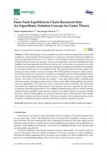
. COMPARISON BETWEEN THE PROPOSED INERATIVE PROCEDURE AND NON -LINEAR FORMULATION At this point, the reasons for developing the iterative procedure utilizing the pre-processor and the modified linear formulation instead of using the complete non-linear formulation will be discussed. First of all, the iterative procedure is guaranteed to yield the solution, while the non-linear formulation may or may not give the solution. Morever, the solution by non-linear formulation could be just one of many local solutions. Secondly, the iterative procedure does not need the initial guess while the non-linear formulation needs a very good initial guess on all the variables. Thirdly, the algorithm for the iterative procedure is definite and concise. Its codes can be easily written by the user while the effective algorithm should be provided for the non-linear formulation. Finally, the iterative procedure is much more efficient than the non.linear formulation in terms of time, if a good initial guess cannot be given for the non-linear optimization. I such a case, the search may progress for a very long time.
A grid with 80 square elements is used to discretize the circular contact area. The following values are given :
M=O.3N.m, f =O.1 The influence coefficients are calculated by using the solution for a semi-infinite body subjected to a tangential force since the radius of the circular contact area is small in comparison with the radii of the spheres in contact(Love, 1944). A comparison between Lubkin's theory(solid line) and the numerical results(symbol o) is plotted in Fig. 3, and good agreement can be seen. The rigid body rotation(0.10641 • 10-2 rad) is also found to compare favorably with Lubkin's theory
L
f2=0.]2
6. I L L U S T R A T I V E
Contact stresses on circular contact area
P2=70 MPa
EXAMPLES
55 N-m ]~) fl=0.12
6.1 C i r c u l a r H e r t z i a n
p] =]40 MPa
Contact
The frictional contact between a steel sphere(E = 207 GPa, u = 0.3) with a radius of 25mm on a steel sphere of the same radius is selected as an example for comparison with the analytical solution by Lubkin(Lubkin, 1951). According to the Hertz theory, the applied normal load of 9600N forms the circular contact area of radius a and the contact pressure d i s t r i b u t i o n p, the m a g n i t u d e s of which are as follows(Johnson, 1985) : a = 0.93mm, p = 531011- (r/a) 2]~12MPa
Index
A B C D E F
Fig. 4
Stress (MPa} 2.75 5.50 8.25 Ii.00 13.75 ]6.50
I
Magnitude of stress on discrete contact area
~%-_ ~_
A N ALGORITHMIC SOLUTION FOR FRICTIONAL CONTACT PROBLEMS SUBJECTED TO A TWISTING MOMENT 113 -i
I
I 1
I
-130. !
I
~
-120.
-120.
-170.
-II0.
-160.
-150 .
-100.
-t50.
L ....
-140.
f2=0, [2 P2=70 MPa
P2=70 MPa 55 N.m ~)
f]=O.]2
~0. 20.
Fig. 5
I
-170.
-140. f2=0.12
-
-130.
-]10.
-100.
--
55 N-m ~)
p ] = ] 4 0 MPa
30.
f1=0.12
p]=]40 MPa
60.
60.
50.
50.
40.
Direction of stress on discrete contact aree(degree)
~0.
Fig. 7
20.
30.
40.
Direction of stress on discrete contact area using NLP(degree)
(0.11119x 10⁻²rad), with a deviation of 4.30%.
6.2 D i s c o n n e c t e d Bodies
Contact
Areas
on Semi-Infinite
Two disconnected square contact areas of the same size(15mm • 15mm) semi-infinite steel bodies(E = 207 GPa, u = 0.3) are considered in this case. Uniform pressure is assumed on each contact region(p~ = 140MPa,p~= 70MPa). The coefficient of friction on both region 1 and region 2 is assumed to be the same (A=f2=0.12). The twisting moment is taken as 55 N" m. Since the contact regions are assumed on semi-
f2=0.12
infinite bodies, the solution for a semi-infinite body subjected to a tangential force is again employed to obtain the influence coefficients(Love, 1944). The contours of the magnitude and the direction of the traction using the proposed iterative procedure are shown in Figs. 4. and 5. As would be expected, different traction distributions are shown in the two regions, and the center of rotation is consequently found to be displaced from the centroid. Three iterations were necessary and the CPU time elapsed was 2 minutes and 59 seconds on a HARRIS 800. The contour plots for the corresponding results using the non-linear programming are also shown in Figs. 6 and 7. When the results of the modified linear programming with the centroid as the center of rotation were used as a set of initial guesses for nonlinear programming, the CPU time used was 8 minutes and 56 seconds. The results using the proposed method compare favorably with those using the non-linear programming. The location of the center of rotaion with respect to the centroid is plotted versus the applied twisting moment in Fig. 8. The development of the slip region with the increasing
P2=70 MPa
~ ) 55 N-m
8 E
fl=0.12
7
pl=140 MPa
6 5
Index A B C D
E F
Fig. 6
Stress (MPa) 2.75 5.50 8.25 II.00 ~3.75 16.50
1
Magnitude of stress on discrete contact area using NLP
o~ u_
o
G~
4
3 2
z u 0
.
=
Io
0
10
2O
40
r
SO
70
W
TNISTING t40WENT (N-m) Fig. 8
Location of center rotation w.r.t, centroid
114
Dong Hoon Choi
]
2
2
3
3
2
2
~
4
4
4
3
2
4
5
5
5
4
0 "~
3
4
5
5
5
5
z ~
4
i 5
5
5
5
5
5
5
z Ud 40
i
2
3 [ f2=O. ] 2
0
4
2
p2: 70M[~.~
|
4
6
8
10
12
14
ANGLEOF TWIST (XI[34 tad} f]:O.]2
Pi:140 MPa
Fig. 10
7
7
7
7
6
5
7
7
7
7
6
5
7
7
7
7
6
5
6
7
7
7
6
5
6
6
6
6
6
5
5
5
5
5
5
3
Twisting moment-angle of twist curve
has proved its accuracy by comparison with Lubkin's theory. The method has been successfully applied to the case of an asymmetric contact area to demonstrate its versatility. The proposed technique seems to be a general and effective procedure for the solution of this class of contact problem.
REFERENCES 33
Fig. 9
44
55
66
77
85
87
N-m
Development of slip on discrete contact area with increased twisting m o m e n t
twisting moment is shown in Fig. 9. The numbers(i,2,3,...,7) refer to the order of the progression of slip when the corresponding twisting moments(33,44,...,87 N" m) are increasingly applied. The curve relating the angle of twist and the twisting moment is plotted in Fig. 10.
7. CONCLUSION A relatively simple technique has been suggested to solve a frictional contact problem subjected to a twisting moment between two elastic non-conforming bodies. The application of the method to the contact problem between two spheres
Cattaneo, C., 1938, "Sul contatto di due corpi elastici : distribuzione locale degli sforzi", Accademia Lincei, Rendiconti, Series 6, Vol. 27, pp. 342-348, 434-436, 474-478. Conry, T.F. and Seireg, A.A., 1971, "A Mathematical Programming Method for Design of Elastic Bodies in Contact", J. of Appl. Mech. Vol. 93, pp. 387-392. Deresiewicz, H., 1952, "Contact of Elastic Spheres under an Oscillating Torsional couple," J. of Appl. Mech., Vol. 76, pp. 52-56. Het~nyi, M. and McDonald, H., 1958, "Contact Stresses under Combined Pressure and Twist", J. of Appl. Mech., Vol. 80, pp. 396-410. Johnson, K.L., 1985, Contact Mechanics, Cambridge Univ. Press, pp. 92-93. Love, A.E.H., 1944, A Treatise on the Mathematical Theory of Elasticity, Dover Book Company, Art. 166. Lubkin, J.L., 1951, "The Torsion of Elastic Spheres in Contact", J. of Appl. Mech., Vol.73, pp. 183-187. Mindlin, R.D, 1949, "Compliance of Elastic Bodies in Contact," J. of Appl. Mech., Vol. 71, pp. 259-268.