Finite element algorithms for contact problems - Springer Link

Vol. 2, 4, 1–49 (1995)

Archives of Computational Methods in Engineering State of the art reviews

Finite Element Algorithms for Contact Problems P. Wriggers Institut f¨ ur Mechanik, TH Darmstadt D-64289 Darmstadt, Hochschulstrasse 1, Germany

Summary The numerical treatment of contact problems involves the formulation of the geometry, the statement of interface laws, the variational formulation and the development of algorithms. In this paper we give an overview with regard to the different topics which are involved when contact problems have to be simulated. To be most general we will derive a geometrical model for contact which is valid for large deformations. Furthermore interface laws will be discussed for the normal and tangential stress components in the contact area. Different variational formulations can be applied to treat the variational inequalities due to contact. Several of these different techniques will be presented. Furthermore the discretization of a contact problem in time and space is of great importance and has to be chosen with regard to the nature of the contact problem. Thus the standard discretization schemes will be discussed as well as techiques to search for contact in case of large deformations.

1. INTRODUCTION Boundary value problems involving contact are of great importance in industrial applications in mechanical and civil engineering. The range of application includes metal forming processes, drilling problems, bearings, crash analysis of cars, car tires or cooling of electronic devices. Other applications are related to biomechanics where human joints, implantats or teeth are of consideration. Due to this variety contact problems are today combined either with large elastic or inelastic deformations including time dependent responses. Thermal coupling might have to be considered, see the cooling of electronic devices, the heat removal within nuclear power plant vessels or thermal insulation of astronautic vehicles. Even stability behaviour has to be linked to contact, like wrinkling arising in metal forming problems. Due to this technical importance a great number of researchers have investigated contact problems. In the ancient egypt people needed to move large stone blocks to build the pyramids and thus had to overcome the frictional force associated with it. Thus many known researchers in the past have investigated frictional contact problems, amongst them were Da Vinci, Amontons, Newton, Coulomb. Their investigations were based on the assumption of rigid bodies. Starting with the classical analytical work of Hertz (1882) on the elastic contact of two spheres the deformation of the bodies being in contact has been taken into account. However only very few problems involving contact can be solved analytically. Thus for most industrial applications numerical methods have to be applied when the contacting bodies have complex geometries . Due to that the solution of contact problems with finite element methods has a relatively long history, see Wilson, Parsons (1970) or Chan, Tuba (1971) for early treatments. In this overview article we will restrict ourselves mainly to finite element techniques for the treatment of contact problems despite many other numerical schemes and analytical approaches could be discussed as well. Furthermore we like to note that the description of the mechanical behaviour of the bodies coming into contact will not be investigated in detail, although this is of great importance. This article thus concentrates on the behaviour in the contact interface. The associated formulation and discretization within the finite element method will be considered as well as the development of algorithms.

c 1995 by CIMNE, Barcelona (Spain).

ISSN: 1134–3060

Received: March 1995

2

P. Wriggers

The following introductory remarks are related to the steps which have to be followed when treating contact problems within the finite element method. 1. 2. 3. 4. 5. 6. 7.

Continuum based contact kinematics, Constitutive equations for contact interfaces, Weak form of contact contributions and overall solution strategies for contact problems, Discretization of contact surfaces, Algorithms for the integration of constitutive equations in the contact area, Contact search algorithms, Adaptive methods for contact problems.

1. Contact kinematics. Since the contact area is not known a priori, and depends in a nonlinear way on the loading, contact problems are nonlinear even for linear elastic solids. Furthermore many technical contact problems involve also large deformations of the bodies being in contact; thus we will formulate all contact relations for finite deformations. In general two steps have to be followed to set up the contact geometry: the search for contact and development of the local kinematical relations. Here we will focus on the local kinematical relations, searching algorithms are discussed later, see part 6. In a large deformation, continuum based formulation of contact kinematics the distance between the bodies being in contact is minimized as can be found for the classical non–penetration condition in e.g. Alart, Curnier (1988). In case that a small penetration due to the approach of the two bodies in contact has to be allowed the contact kinematics are developed in Wriggers, Miehe (1992). This non–penetration function plays also a significant role for the definition of the tangential velocity in the contact interface which is needed to formulate frictional problems, see e.g. Simo, Laursen (1992), Wriggers, Miehe (1992), Laursen, Simo (1993), Wriggers, Miehe (1994) or Klarbring (1994). 2. Constitutive equations for contact interfaces. Due to the precision which is needed to resolve the mechanical behaviour in the contact interface, different approaches have been used in the literature to model the mechanical behaviour in contact area. Two main lines can be followed within the finite element method to impose contact conditions in normal direction. These are the formulation of the non–penetration condition as a purely geometrical constraint and the development of constitutive laws for the micromechanical approach within the contact area. The first formulation is in general used for problems with “low contact precision” where the most essential necessity is the correct enforcement of the geometrical constraints like in crash or forming simulations. In this case it is not possible to specify constitutive relations in the contact interface. Here the normal contact pressure is related to the reaction in the contact area and can be deduced from the constraint equations. This procedure is the classical way to formulate contact constraints; thus numerous researcher have used this strategy. For applications using the finite element method we like to mention the early work by Wilson, Parsons (1970) or Chan, Tuba (1971) for small deformation problems or the work by Alart, Curnier (1988) for large deformations. However, as discussed before, there exist also contact problems where the knowledge of the micromechanical approach is essential for a proper treatment of the physical phenomena. Then interface compliances are needed for these problems with “high contact precision”. Constitutive equations for the normal contact can be developed by investigating the micomechanical behaviour within the contact surface. Associated models have been developed based on experiments, see e.g. Greenwood, Williamson (1966) or Kragelsky, Dobychin, Kombalov (1982). The micromechanical behaviour depends in general on material parameters like hardness and on geometrical parameters like surface roughness. It should be noted that the real micromechanical phenomena are extremly complex: due to

Finite Element Algorithms for Contact Problems

3

very high local pressures, e.g. in the case of an impact, chemical reactions can be initiated in the interface by the mechanical forces. The models which are used try only to capture the most important phenomena and assume either an elastic or a plastic deformation of the asperities being in real contact in the interface. The interfacial behaviour in the tangential direction (frictional response) is even more complicated. Some researchers try to formulate a third body in the interface which has special properties and is only present in the moment of the tangential mechanical loading, see Kragelsky (1956). We will here restrict ourselves to more simple formulations which yield constitutive equations for frictional contact as long as one does not assume perfect stick within contact area. The most frequently used constitutive equation is the classical law of Coulomb. However, other frictional laws are available which take into account local, micromechanical phenomena within the contact interface, see e.g. Woo, Thomas (1980). An extensive overview may be found in Oden, Martins (1986). The main governing phenomena are adhesion of the surfaces and ploughing of the asperities. For the physical background see e.g. Tabor (1981). During the last years frictional phenomena have also been considered within the framework of the theory of plasticity. This leads to non–associative slip rules, different relations have been proposed for frictional problems by e.g. Bowden and Tabor (1964) and Michalowski, Mroz (1978). Further discussion is contained in Curnier (1984). The application of constitutive equations for friction within finite element calculation can be found in e.g. Fredriksson (1976), Wriggers, Vu Van, Stein (1990). In cases where thermomechanical contact has to be considered, a “high contact precision” formulation must be applied to account correctly for the pressure dependency of the heat conduction in the contact area. This is due to the fact that the heat conduction depends on the approach of the two rough surfaces being in contact, see section 3.3. In this context models have been discussed for the onstitutive behaviour in normal direction on the basis of statistical methods, see e.g. Cooper, Mikic, Yovanovich (1969) or Song, Yovanovich (1987). A finite element treatment for thermomechanical contact problems can be found in Zavarise (1991), Zavarise, Wriggers, Stein, Schrefler (1992a,b) and in combination with frictional heating in Wriggers, Miehe (1994). Also other contact phenomena like wear, see e.g. Johannson, Klarbring (1992), need special constitutive laws which have to be developed in the interface. 3. Weak form of contact contributions and overall solution strategies. The weak formulation of contact problems leads to variational inequalities, see Duvant, Lions (1976) since contact conditions are represented as inequality constraints. Different possibilities exist for the numerical solution of these problems. Among them are the so called active set strategies which are applied in combination with Lagrangian multiplier or penalty techniques, see e.g. the text books of Bertsekas (1984) or Luenberger (1984); these methods are well known in optimization theory. Other solution schemes are based on mathematical programming, see e.g. Conry, Seireg (1971) or Klarbring (1986), who applied this method to frictional contact problems. Most standard finite element codes which are able to handle contact problems use either the penalty or the Lagrangian multiplier method, for an overview and the mathematical framework, see e.g. Kikuchi, Oden (1988). Each of the methods has its own advantages and disadvantages which will be discussed in detail in the following. The methods are designed to fulfill the constraint equations in normal direction in the contact interface. For the tangential part we need in general constitutive relations; associated techniques will be discussed later. A combination of the penalty and the Lagrangian multiplier technique leads to the so called augmented Lagrangian methods which try to combine the merits of both approaches. A general discussion of these techniques can be found in Glowinski, Le Tallec (1984) and with special attention also to inequality constraints in Bertsekas (1984). However this technique requires an algorithmic treatment, the Uzawa method, which increases the total number of

4

P. Wriggers

iterations. For applications of augmented Lagrangian techniques to contact problems within the finite element method, see e. g. Wriggers, Simo, Taylor (1985), Simo, Laursen (1992) or for a symmetrical treatment of the frictional part Laursen, Simo (1993b) or Zavarise, Wriggers, Schrefler (1995). In the case of ”high precision contact”, when constitutive interface laws are employed, special augmented Lagrangian techniques are needed, since often ill–conditioning of the problem may occur, see Wriggers, Zavarise (1993). In case of thermomechanical contact problems two fields – deformation and temperature – interact and thus have to be considered within the formulation. In the general setting these fields are coupled since the constitutive parameters depend on the temperature, the evolution of the thermal field is related to the deformation and heat can be generated by dissipative mechanisms like plastic deformations or frictional forces. The technical importance of these models has lately raised some interest in these phenomena, thus many contributions can be found in the literature. Here we discuss only the research which is directly related to the numerical treatment of contact problems within the finite element method. A finite element model based on micromechanical interface laws is derived in e.g. Zavarise, Wriggers, Stein, Schrefler (1992) for finite deformations. Wriggers, Zavarise (1993) have developed a simple element for the case of small deformations. In both approaches a global iterative procedure has been used for a stationary process. Staggered schemes, which treat the deformation and temperature fields seperately can be computationally more advantageous, see Wriggers, Miehe (1994) for thermomechanical contact and Simo, Miehe (1992) for thermomechanical problems without contact. 4. Discretization of the contact surfaces. When the discretization of contact surfaces is concerned one has to distinguish between the contact of two deformable bodies or the contact of a deformable body with a rigid obstacle. On a first glance it seems that the latter case is simply a special case of the first problem, which is true. But due to the fact that the surface description of a rigid obstacle can be given once and for all by the correct geometrical model this knowledge can be used within the discretization process. Hansson, Klarbring (1990) have developed a formulation based on CAD–surfaces, Williams, Pentland (1992) considered so called superquadrics to specify the geometry of contacting objects and Wriggers, Imhof (1993) formulated the contact problem with splines. In the first applications of finite elements to contact problems of two deformable bodies only small changes in the geometry were assumed so that the geometrically linear theory could be applied. Then it is possible to incorporate the contact constraints on a purely nodal basis, see e.g. Francavilla, Zienkiewicz (1975). Later also contact elements were developed which resulted from a degenerated solid element, see e.g. Stadter, Weiss (1979) or the textbook of Kikuchi, Oden (1988). A mathematical study of these classes of elements which also accounts for the correct integration rules can be found in Oden (1981). All of the above mentioned elements need a discretization in which the element nodes match each other in the contact interface. For the general case of nodes being arbitrary distributed along the possible contact interface between two bodies, which can occur when automatic meshing is used for two different bodies, Simo, Wriggers, Taylor (1984) developed a segment approach to discretize the contact interface. For the general case of contact including large deformations the most frequently used discretization is the so called node–to–segment approach. Here arbitrary sliding of a node over the entire contact area is allowed. Early implementations can be found in Hallquist (1976) or Hughes, Taylor, Kanuknukulchai (1978) which have been developed for more and more general cases, Hallquist, Goudreau, Benson (1983), Bathe, Chaudary (1985) and Wriggers, Vu Van, Stein (1990). Now some finite element codes include also self–contact, see Hallquist, Schweizerhof, Stillman (1992). Also the idea of contact segments proposed by Simo, Wriggers, Taylor (1984), has been followed up and applied to problems involving large deformations, see Papadopoulos, Taylor (1992).


5

A consistent linearization is needed within Newton procedures to solve the nonlinear contact problems incrementally. For a discretization using the node–to–segment approach Wriggers, Simo (1985) derived for two–dimensional large deformation problems the needed matrix formulation under the assumption of frictionless contact. The formulation for frictional contact can be found in Wriggers, Vu Van, Stein (1990). The associated tangent matrices for the frictionless three–dimensional case of a node–to–surface discretizations is developed in Parisch (1989). The special case of the contact of a body with a rigid obstacle is treated in Hansson, Klarbring (1990), Wriggers, Imhof (1993) or Heegard, Curnier (1993). The consistent linearization for a continuum based approach to contact problems has been derived in Laursen, Simo (1993a). 5. Algorithms for the integration of constitutive equations in the contact area. In general we have to distinguish three cases of constitutive equations in the contact interface. These are related to the normal, the tangential and the thermal part of the contact. For the normal contact a mere function evaluation –like for finite elasticity– can be used to obtain for a given approach the contact pressure; even if the micromechanical derivation of the contact compliance involves plastic deformations. This is theoretically not satisfactory but up to now – due to the extremely complex behaviour in the contact interface – the only possible method for the macroscopic description of normal contact compliance. The situation is different for friction. Then one has to solve an evolution equation for the frictional slip which needs special algorithms. In early finite element applications often so–called ”trial–and–error” algorithms have been applied, see e.g. (19), which might not converge in some cases. More reliable methods are provided by the mathematical programming approach, Klarbring (1986). Another way which is now becoming more and more standard for numerical simulations involving friction is related to the possibility to recast the fricional interface laws in terms of non–associated plasticity. First formulations and applications in finite element analysis are found in Fredriksson (1976). A theoretical basis was also provided by Michalowski, Mroz (1978). The major break through in terms of convergence behaviour and reliability of the solution algorithms came with the application of the return mapping schemes to frictional problems. Its application can be found in Wriggers (1987) or Giannokopoulos (1990) for geometrically linear problems. This approach provides the possibility to develop algorithmic tangent matrices which are needed to achieve quadratic convergence within Newton–type iterative schemes. Due to the non–associativity of the frictional slip these matrices are non–symmetrical. For the case of large deformations associated formulations have been developed in Ju, Taylor (1988) for a regularized Coulomb friction law and in Wriggers, Vu Van, Stein (1990) for different frictional laws formulated in terms of non–associated plasticity. A three–dimensional formulation can be found in Laursen, Simo (1993a) who also developed an algorithmic symmetrization (Laursen, Simo (1993b)), see also Zavarise, Schrefler, Wriggers (1995). 6. Contact search algorithms. The search for the active set of contact constraints is not trivial in case of large deformations since a surface point of a body may contact any portion of the surface of another body. Such point can even come into contact with a part of the surface of its own body. Thus the search for the correct contact location needs, depending on the problem, eventually considerable effort. An implementation where each node of a surface is checked against each element surface in the mesh is too exhaustive and thus computationally inefficient and refined algortihms have to be constructed. This especially true when the contact of more then two bodies has to be considered or when self–contact is possible. The development of search algorithms can be split in two general approaches. The first is connected with the contact between a deformable and a rigid body. In this case the rigid body can be described by implicit functions such as superquadrics or hyperquadrics, see

6

P. Wriggers

Williams, Pentland (1992). This leads to a simple and efficient contact check for points lying on the surface of the deformable body. For the special case of cylinders or ellipses see also e.g. Hallquist, Schweizerhof, Stillman (1992). In case that two or more deformable bodies contact each other or that self–contact of one body occurs the search algorithms are more complex and normally split into a global and a local search. Within the global search a hierarchical structure can be set up to find out which bodies, parts of the bodies, surfaces or parts of the surfaces are able to come into contact within a given time step or displacement increment, see e.g. Zhong, Nilsson (1989), Zhong (1993) or Williams, O’Connor (1995). Different methods can be applied to determine the possible contact partners. Lately a considerable impact has come from discrete finite element methods where several thousand particles have to be included in the contact search. Methods like space cell decomposition have been considered by Belytschko, Neal (1989) a combination with binary tree search can be found in Munjiza, Owen, Bicanic (1995); whereas Williams, O’Connor (1995) rely on heapsort algorithms for the global search. Once the possible contactors are known the local search is needed to check whether a penetration has occured and to determine its exact location. Different possibilities exist to find the correct finite element surface which is associated with a node that might penetrate through this surface. Here the node–to–segment algorithm Hallquist (1978), the pinball technique, Belytschko, Neal (1991), or methods based on discrete function representation Williams, O’Connor (1995) can be applied among other possibilities. 7. Adaptive methods for contact problems. Since numerical methods for contact problems yield approximate solutions it is necessary to control the errors inherited in the method. During the last ten years research activities have been focused on adaptive techniques providing automatically a numerical modell which is accurate and reliable. The objective of adaptive techniques is to obtain a mesh which is optimal in the sense that the computational costs involved are minimal under the constraint that the error in the finite element solution is beyond a certain limit. Since the computational effort can be linked to the number of unknowns of the finite element mesh the task is to find a mesh with minimum number of unknowns or nodes for a given error tolerance. In general, adaptive methods rely on error indicators and error estimators which can be computed a priori or a posteriori. For an overview over different techniques, see e.g. Johnson (1987) and references therein. Based on the error distribution a new partially refined mesh can be constructed which yields a better approximate solution. To obtain an optimal mesh in the sense of an equal solution quality it is desirable to design the mesh such that the error contributions of the elements are equidistributed over the mesh. During the last years a growing number of papers has been devoted to this topic and applied to problems of solid and fluid mechanics, see e.g. Zienkiewicz, Taylor (1989). The methods rely on error estimators which have been developed so far in different versions. The estimators which are most frequently used in solid mechanics for elastic problems are residual based error estimators, see e.g. Babuska, Rheinboldt (1978) or Johnson, Hansbo (1992), or error estimators which use superconvergence properties, see e.g. Zienkiewicz, Zhu (1987). For frictionless contact problems a priori error estimators have been derived for linear elastic bodies, see e.g. Kikuchi, Oden (1988) or Hlavacek, Haslinger, Necas, Lovisek (1988). An adaptive method for problems with unilateral constraints has been developed by Lee, Oden, Ainsworth (1991) who treated as an example a free surface flow problem. In Wriggers, Scherf, Carstensen (1994) a residual based error estimator has been developed following an approach persued by Johnson, Hansbo (1992) for unilateral membrane problems. But also the Z 2 error estimators, due to Zienkiewicz, Zhu (1987), can be applied to contact problems, see Wriggers, Scherf (1995).


7

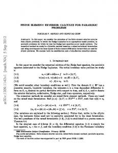
2. CONTACT GEOMETRY This section summarizes relations which are necessary to formulate the geometrical contact conditions. In detail the penetration and the relative slip in the contact area are discussed. The first condition also includes the non–penetration condition which is used classically in contact mechanics. The derivation presented here can be used for frictional or frictionless problems. It follows closely the approach discussed in Wriggers, Miehe (1992) and Wriggers, Miehe (1994). Similar ideas may be found in Laursen, Simo (1993) or for the frictionless case in Curnier, Alart (1992). We assume that two bodies which undergo large deformations can come into contact. Let Bγ , γ = 1, 2, denote the two bodies of interest and ϕγt : Bγ → IR3 the associated deformation maps at time t ∈ IR+ . ϕγt maps points Xγ ∈ Bγ of the reference configuration onto points xγ = ϕγt (Xγ ) of the current configuration. Motivated by micromechanical investigations of contact problems we view the mechanical approach of the two contact surfaces as a microscopical penetration of the current mathematical boundaries ϕγt (Γγc ). Note that we can recover the non–penetration condition as a limiting case. In this formulation Γγc ⊂ ∂Bγ are possible contact surfaces of the bodies Bγ , see Figure 1 for an illustration of this concept. In what follows we denote ϕ1t (Γ1c ) as the current slave surface which penetrates in the case of contact into the current master surface ϕ2t (Γ2c ). The latter one plays within our formulation of the contact geometry the role of a (moving) reference surface. We parametrise the master surface in its reference and current configuration by the natural parameters ξ 1 , ξ 2 , i.e. we consider material curves ˆ 2 (ξ 1 , ξ 2 ) ⊂ Γ2 and x2 = x ˆ 2t (ξ 1 , ξ 2 ) ⊂ ϕ2t (Γ2c ). Then the local deformation gradient X2 = X c of the master surface is given by F2t := a2α ⊗ A2α based on the tangent vectors of the contact ˆ 2 (ξ 1 , ξ 2 ) with the standard relations a2 · a2β = δβ ˆ 2t,α (ξ 1 , ξ 2 ) and A2α := X surface a2α := x ,α α α and A2α · A2β = δαβ and ( ),α denotes differentiation with respect to ξ α .

Figure 1. Contact geometry and geometrical approach

8

P. Wriggers

2.1 Penetration As the first relevant function for the contact geometry we define a penetration function on the current slave surface ϕ1t (Γ1c ) by setting, see Wriggers, Miehe (1992) ˆ 2t (ξ¯1 , ξ¯2) for [ x1 − x ˆ 2t (ξ¯1, ξ¯2 ) ] · n ¯2 < 0 . x1 − x (1) gN + = 0 otherwise Here (ξ¯1 , ξ¯2 ) is the minimizer of the distance function for a given slave point x1 ˆ 2t (ξ 1 , ξ 2 ) −→ MIN . dˆ1 (ξ 1 , ξ 2 ) = x1 − x

(2)

The values (ξ¯1 , ξ¯2 ) are obtained by writing the necessary condition for the minimum of the distance function (2) ˆ 2t (ξ 1, ξ 2 ) x1 − x d ˆ1 1 2 ˆ 2 (ξ 1, ξ 2 ) = 0 . ·x d (ξ , ξ ) = ˆ 2t (ξ 1, ξ 2 ) t,α dξ α x1 − x

(3)

The solution of (3) requires the orthogonality of the first and second term. Since ˆ 2t,α (ξ 1 , ξ 2 ) is the tangent vector a2α the first term must denote the normal n2 . Thus we x ˆ 2t (ξ 1, ξ 2 ) is have the condition −n2 · a2α = 0 which means that the current master point x 1 the orthogonal projection of a given slave point x onto the current master surface ϕ2t (Γ2c ). Here and in the following we will denote by a bar over a quantity its evaluation at the minimal distance point (ξ¯1, ξ¯2 ) which means that these values denote the solution point of ¯ 2 := (¯ ¯22 ) / ¯ ¯22 is the outward unit normal on the current master (3). Thus n a21 × a a21 × a ˆ 2t (ξ¯1 , ξ¯2 ). ¯2α are tangent vectors at x surface at the master point where a The penetration function (1) contains two informations: 1. gN + serves as a local contact check, i.e. we set: contact ⇔ gN + > 0 2. gN + enters for gN + > 0 as a local kinematical variable the constitutive function for the contact pressure. By taking the time derivative of (2) at the minimal distance point (ξ¯1 , ξ¯2 ) one obtains, in the case of contact, the rate of penetration ˆ t2 (ξ¯1 , ξ¯2 ) ] · n ¯2 g˙ N + = [ vt1 − v

(4)

ˆ 2t (ξ¯1 , ξ¯2 ) at the slave and master points. for given spatial velocities vt1 and v REMARK I: L 1 ˆ 2t (ξ¯1 , ξ¯2 ) ] · n ¯ 2 ≥ 0 represents the classical non–penetration condition for 1. gN + = [x − x finite deformation. 2. The time derivative of the penetration function (4) can be viewed as the variation of (2) when the velocities are exchanged by the associated variations leading to

¯2 δgN + = [ η 1 − ηˆ2 (ξ¯1 , ξ¯2) ] · n

(5)

with η being the virtual displacement or test function. 3. For the analysis of small deformation problems the kinematical relation (1) or the non– penetration condition from Remark I.1 can be linearized which yields ¯ 2 + g0 ˆ 2 (ξ¯1 , ξ¯2 ) ] · N ∆gN + = [ u1 − u

(6)

uγ represents the displacement field which is introduced in the kinematically linear case to connect the current and the reference configuration via: xγ = Xγ +uγ . The variable g0

9


ˆ 2 (ξ¯1 , ξ¯2 )]· N ¯2 denotes the initial gap between the two bodies which is given by g0 = [X1 − X 2 2 2 2 2 ¯ = (A ¯ ×A ¯ ) / A ¯ ×A ¯ is related to the reference configuration. and the normal N 1 2 1 2 2.2 Tangential Relative Velocity and Tangential Relative Slip The tangential relative slip between two bodies is related to the change of the solution point (ξ¯1 , ξ¯2 ) of the minimal distance problem. Thus we can compute the time derivative of ξ α from (3). This yields the following result d 2 ˆ 2t (ξ¯1 , ξ¯2 ) ] · a ¯2α } = [ vt1 − v ˆ t2 (ξ¯1 , ξ¯2 ) − a ¯2β ξ¯˙β ] · a ¯2α + [ x1t − x ˆ 2t (ξ¯1 , ξ¯2 ) ] · a ¯˙ α = 0 (7) { [ x1t − x dt 2 2 ¯˙ α = v ˆ t,α ˆ 2t,αβ (ξ¯1, ξ¯2 ) ξ¯˙β we obtain ξ¯˙β from the following system of equations with a (ξ¯1 , ξ¯2 ) + x

¯α ¯ αβ ξ¯˙β = R H

(8)

¯ αβ = [ a H ¯αβ + gN + ¯bαβ ] , 2 ¯ α = [ v1 − v ˆ t2 (ξ¯1, ξ¯2 ) ] · a ¯2α + gN + n ˆ t,α ¯2 · v R (ξ¯1, ξ¯2 ) . t

(9)

with

a ¯αβ and ¯bαβ are the first and second fundamental form of the deformed surface, well known from differential geometry. Let us now define the tangential relative velocity function on the current slave surface ϕ1t (Γ1c ) by setting ¯2α . Lv gT := ξ¯˙α a

(10)

Equation (10) determines per definition the evolution of the tangential slip gT which enters as a local kinematical variable the constitutive function for the contact tangential stress, see next section. The rate ξ¯˙α in (10) at the solution point (ξ¯1 , ξ¯2 ) has been already computed in (8). REMARK II: ¯ αβ and R ¯ α of (9) depend on the penetration gN + . In the 1. Note that the last terms in H case of a strong enforcement of the non–penetration condition (gN + = 0) with Lagrangian multipliers these terms vanish. Then the evolution Lv gT in (10) is given by the projection ¯ evaluated at the slave and master points onto the ˆ t2 (ξ) of the spatial velocities vt1 and v tangential direction of the master surface at the master point: ¯ T [ vt1 − v ˆ t2 (ξ¯1 , ξ¯2 ) ] , Lv gT := P

with

¯T = a ¯2α ⊗ a ¯2α . P

2. If the deformed contact surface is flat then the curvature tensor ¯bαβ is zero. This is always the case for a surface discretization by three node triangular elements. 3. Note that the (a priori objective) Lie derivative of the tangential vector gT has the d ¯α based on the deformation gradient F2t [F2−1 (gT ) ] } = ξ¯˙α a representation Lv gT = F2t { dt t of the master surface defined above. Thus (10) represents an evolution equation for the objective rate Lv gT of the tangential vector introduced above. 4. In case of no relative movement in tangential direction (stick condition) we have Lv gT = gT = 0.

10

P. Wriggers

5. In the geometrically linear case we obtain from (7) and (6) d ¯ 2 } = [ v1 − v ¯ 2 ξ¯˙β ] · A ¯2 ˆ 2t (ξ¯1, ξ¯2 ) ] · A ˆ t2 (ξ¯1 , ξ¯2 ) − A { [ x1t − x β α t α dt which yields

¯2 ˆ 2t (ξ¯1 , ξ¯2 ) ] · A A¯2αβ ξ¯˙β = [ vt1 − v α

The terms multiplied by gN + can be neglected. Thus ξ¯˙β is given by the projection of the difference velocity of the two bodies at the contact point on the tangent direction of the undeformed surface. From the last equation we can deduce the the relative tangential ¯2. velocity at the contact point: g˙ T = ξ¯˙β A α 3. CONSTITUTIVE EQUATIONS FOR CONTACT INTERFACES As discussed in the introductory remarks, the normal contact stresses can be obtained in two generally different ways. On one hand the contact stresses follow from the constraint equations. On the other hand an approach of both bodies is observed in the contact area which then leads to the formulation of associated constitutive interface equations. 3.1 Normal Stress in the Contact Area In the first case the mathematical condition for non–penetration is stated in remark I.1 as L gN + ≥ 0 which precludes the penetration of one body into another. Then contact takes L place when gN + is equal to zero. In this case the associated normal components pN of the ¯ + tβ a ¯ β in the contact interface must be non–zero. The stress vector stress vector t = pN n acts on both surfaces, obeying the action–reaction principle: t2(ξ¯1 , ξ¯2 ) = −t1 in the contact point x1 . We have pN = p1N = p2N < 0 since adhesive stresses will not be allowed in the contact interface. This leads to the statement L gN + ≥ 0,

pN ≤ 0 ,

L pN gN + = 0

(11)

which is well known as the Kuhn–Tucker condition for frictionless contact problems. These conditions provide the basis to treat contact problem in the context of constraint optimization. For further details see the next section. When the micromechanical behaviour of the contact area is studied different phenomena have to be considered for the mechanical interface description. Here we restrict ourselves to constitutive models which have been derived based on micromechanical observations of physical contact surfaces. These models can be related to formulations relative to mathematical contact surfaces by an averaging process as symbolically indicated in Figure 2. Goal of this section is to formulate local constitutive equations for the pressure and the ¯ 2 } acting on tangential stress on the slave surface at point x1 relative to the bases {¯ a2α , n 1 body B . It is well known that the contact pressure is related to the approach of the physical surfaces which come into contact, i.e. the penetration of the mathematical surfaces results from the deformation of the micro–asperities, see Figure 3. Let us assume the following general form of the constitutive law pN = f (d)

or

d = h (pN )

(12)

where f and h are nonlinear functions of the current mean plane distance d or the contact pressure pN , respectively.


11

Figure 2. Averaging of micromechanical contact relations

Figure 3. Physical approach in Γc

Most of the interface laws can be written in the form (12). Out of many different possibilities two constitutive equations for normal pressure in the contact area will be stated. The first was developed in Zavarise (1991), Zavarise, Schrefler, Wriggers (1992), and is based on a statistical model of the microgeometry proposed by Cooper, Mikic, Yovanovich (1969), recently revisited in Song, Yovanovich (1987). σ c2 c1 1617646.152 m 1 + 0.0711 c2 2 pN = (13) exp − d . 2 5.5891+0.0711 c2 (1.363σ) Here c1 and c2 are mechanical constants expressing the nonlinear distribution of the surface hardness, σ and m are statistical parameters of the surface profile, representing the RMS surface roughness and the mean absolute asperity slope. Thus we have an exponential law 2 of the form pN = c3 e−c4 d .

12

P. Wriggers

In case of contact the current mean plane distance is related to the geometrical approach gN + (1) as follows (14) gN + = ζ − d where ζ is the initial mean plane distance in the contact area Γc . Another law for the contact pressure has been given, based on experimental investigations, by Kragelsky, Dobychin, Kombalov (1982). These authors formulated the following nonlinear elastic constitutive equation for the contact pressure pN = cN ( gN + )n

(15)

in terms of the penetration gN + defined in (1). Here cN and n are material parameters which have to be determined by experiments. 3.2 Tangential Contact Stress and Tangential Frictional Slip Many different constitutive models have been developed to formulate the interfacial behaviour due to friction. In this overview we restrict our consideration to two models for frictional behaviour; one being the classical Coulomb model. The response in tangential direction can be divided in two different actions. In the first no tangential relative displacement of the two bodies occurs which is the so–called stick condition. The second action is associated with a relative tangential movement in the contact interface which denotes the so–called slip. The stick condition can be formulated with remark II.4 simply as gTL = 0

(16)

which imposes in general a nonlinear constraint equation on the motion in the contact interface. Associated with this constraint is a Lagrangian multiplier, λ T , which denotes the reaction due to (16). In case of sliding the law of Coulomb yields tT = −µ | pN |

Lv gT Lv gT

(17)

where µ is the sliding frictional coefficient which depends on the surface roughness and may also depend on the sliding velocity Lv gT , the pressure pN or the temperature. These and other constitutive equations for friction can be formulated in the framework of elastoplasticity. This has been investigated by several authors who also developed different constitutive equations for frictional problems, see e.g. Michalowski, Mroz (1978) or Curnier (1984). A treatment of frictional interface laws in terms of non–associated plasticity has been considered within a finite element formulation by Wriggers (1987), Giannokopoulos (1989), Wriggers, Vu Van, Stein (1990) or Laursen, Simo (1993). Classically one has to distinguish between stick which means no relative tangential movement in the contact interface and slip which is associated with relative tangential movement. The key idea of the elasto–plastic approach is a split of the tangential slip gT into an elastic part gTe and a plastic (slip) part gTs , see equation (18)2 below. The elastic part describes the micro displacement which can be regarded as stick behaviour since the associated deformations vanish once the loading is removed from the system. The constitutive behaviour for the tangential elastic micro–displacements can be deduced from experiments and is related to the elastic deformation of the asperities due to tangential loading. Here we assume, as the simplest possible model, an isotropic linear elastic constitutive equation for the tangential contact stress tT = cT gTe with gTe := gT − gTs (18)

13


where cT is a material parameter. The tangential plastic slip gTs is governed by a constitutive evolution equation which can be derived by using standard concepts of the theory of elastoplasticity. Within this framework we can formulate a plastic slip criterion function for a given contact pressure pN with material parameter µ which determines the frictional sliding, see Figure 4a, fˆs (tT ) = tT − µ pN ≤ 0 .

(19)

Another slip criterion function has been formulated in Wriggers, Vu Van, Stein (1990) which additionally takes into account the pressure dependency of the tangential response. Here the form µ = τ0 / pr + β proposed by Tabor (1981) for most solids is assumed, where τ0 and β are constitutive parameters and describe a model with linear varying shear strength of the interfacial material due to the true contact pressure. The true pressure pr is related to the true contact area Ar (real contact area due to the contact of the asperities in the contact interface) whereas the pressure pN is associated with the nominal contact area A. Woo, Thomas (1980) have formulated a relation between the true and the nominal area based on experimental observations n | pN | Ar 5 = (20) , n= . A AH 6 with the hardness H of the material. With these relations Wriggers, Vu Van, Stein (1990) arrived at the following slip criterion, see Figure 4b, fˆs (tT , pN ) = tT −α | pN |n −β | pN | ≤ 0 ,

α=

A τ0 . (A H)n

(21)

Note that the choice of one of the slip criteria (19) or (21) has to be made with regard to experimental data within the contact interface; there are of course other slip criteria possible.

Figure 4. a) Coulomb frictional cone; b) Parabolic slip surface

The constitutive evolution equation for the plastic or frictional slip can be stated in form of a slip rule for large deformations in the contact zone as follows Lv gTs = λ

∂ fˆs (tT ) = λ nT , ∂tT

with

nT =

tT tT

(22)

14

P. Wriggers

which denotes a normality rule for a fixed contact pressure pN . Here λ is the plastic parameter which describes the magnitude of the plastic slip. Equations (18), (19) or (20) and (22), along with the loading–unloading conditions in Kuhn–Tucker form λ ≥ 0,

fˆs (tT ) ≤ 0 ,

λ fˆs (tT ) = 0 ,

(23)

establish the constitutive framework for the tangential slip–stick behaviour. The algorithmic treatment will be discussed in section 6. 4. BOUNDARY VALUE PROBLEM, GLOBAL SOLUTION STRATEGIES For the formulation of the boundary value problem we have to discuss only the additional terms due to contact in detail. The equations describing the behaviour of the bodies coming into contact do not change. However, for completeness, the balance equations and a simple constitutive model are stated for elastic solids undergoing finite deformation. 4.1 Local Balance Equations for the Solid We can formulate the local momentum equation for a body Bγ as γ

DIV Pγ + ¯f = 0

(24)

in case that inertia terms are neglected. Pγ denotes the first Piola–Kirchhoff stress tensor γ acting in the body γ, ¯f are the body forces. Next we formulate the boundary conditions for the deformation and the stress field ¯γ ϕγ = ϕ tγ = ¯tγ

on

Γγϕ ,

on

Γγσ

(25)

¯ γ and ¯tγ are described quantities. Furthermore we have to account for the contact where ϕ condition which is given by equation (12)2 with the definition of the gap function (1) when an approach of the bodies in the contact interface is allowed or by the condition defined in remark I.1 which yields the inequality L gN + ≥ 0

on

Γc .

(26)

4.2 Constitutive Relations As a model for non–linear constitutive equations we use a form valid for finite elasticity which leads to a non–linear relation between the Kirchhoff stress τ and the left Cauchy Green tensor b = F FT : τ = f ( b ). The Kirchhoff stress is related to the first Piola–Kirchhoff stress via τ = P FT , with F being the deformation gradient. The simplest constitutive equation for hyperelasticity is known as the Neo–Hookian model and can e. g. be applied for rubber materials undergoing moderately large strains, see e.g. Ogden (1984). It is stated below for the body Bγ with the Jacobian of the deformation J γ = det Fγ τ γ = Λγ ( J γ − 1 ) 1 + µγ ( bγ − 1 ) .

(27)

Material parameters for the body Bγ are the Lamè constants Λγ and µγ . The material model is valid for finite elastic deformations. Of course we can consider more complicated constitutive relations which can also be of inelastic nature. It should be noted that since the contact has to be formulated only within the interface, the constitutive laws for the bodies

15


coming into contact can be arbitrary and do not affect the main algorithmic treatment of the contact problem. However it is clear that the physical properties of the surfaces of the bodies are influenced by the general constitutive behaviour. 4.3 Weak Formulation For a numerical solution of the nonlinear boundary value problem summarized above we will use the finite element method. Thus we need the weak form of equations (24) to (27). Due to the fact that the constraint condition (24) is represented by an inequality we obtain in general a variational inequality. The general form can be written as 2 2 γ γ γ γ γ γ ¯ ¯tγ · (ηη γ − ϕγ ) dA τ · grad (ηη − ϕ ) dV ≥ (28) f · (ηη − ϕ ) dV − γ=1

Ωγ

γ=1

Ωγ

Γσ γ

where the integration is performed with respect to the domain Ωγ occupied by the body Bγ in the reference configuration. The stress tensor and the gradient operator ”grad” are evaluated with respect to the current coordinates. ϕ1 , ϕ2 ) ∈ K such that (26a) is fulfilled for all We now have to find the deformation (ϕ 1 2 (ηη , η ) ∈ K with ¯2 ≥ 0 } , K = { (ηη 1 , η 2 ) ∈ V | [ η 1 − ηˆ2 (ξ¯1 , ξ¯2 ) ] · n see also section 2. In case of finite elasticity the existence of the solution of (28) can be proved, see e.g. Ciarlet (1988) or Curnier, He, Telega (1992). For this, the strain energy function has to be polyconvex and the solution lies in the usual Sobolev space W 1,p . The space V is defined as V = { η γ ∈ [W 1,p (Ωγ )]dim | η γ = 0 on Γu } , dim denotes the dimension of the problem at hand. REMARK III: 1. In the geometrically linear case these equations can be recast in a weak or variational formulation as follows a(u, v − u) ≥ f (v − u) , (29)

with

ε (u) : C 0 : ε(w) dΩ ,

a(u, w) = Ω

ˆ · w dΩ + b

f (w) = Ω

ˆt · w dΓ Γσ

and Ω = ∪γ Bγ . C 0 is the elasticity matrix due to the classical constitutive law of Hooke. The linear strain tensor is defined by ε(u) = 12 (∇u + ∇T u). The problem is now, as in the nonlinear case, to find u ∈ K such that (29) is fulfilled for all v ∈ K with, see equation (6), ¯ 2) · n ¯ 2 + g0 ≥ 0 on Γc } K = {v ∈ V | (v1 − v and

V = {v ∈ [H 1 (Ω)]dim | v = 0 on Γu } .

The mathematical structure of the variational inequality (29) is discused in detail in e. g. Duvaut, Lions (1976) or Kikuchi, Oden (1988). Due to the inequality constraint on the deformation field the contact problem is nonlinear even for the linear elastic case (29).

16

P. Wriggers

Algorithms for solving variational inequalities are given by mathematical programming, active set strategies or sequential quadratic programming methods, to name only a few. Each of these methods which are well known from optimization theory, see e. g. Luenberger (1984), has been applied to contact problems. For mathematical programming see e. g. Conry, Seireg (1971) or Klarbring (1986). The sequential quadratic programming approach has been considered by e.g. Barthold, Bischoff (1988) and lately with application to large strain elasticity by Bj¨ orkman, Klarbring, Sj¨ odin, Larsson, R¨ onnqvist (1995). Here we will investigate in more detail the active set strategies which are applied in many existing finite element codes. Within this method the contact constraints can be introduced via Lagrangian multipliers or penalty terms. Furthermore we will observe that the introduction of a constitutive equation for the normal approach in the contact interface, see section 3.1, yields a formulation which is like a nonlinear penalty method. Within an active set strategy we can write the weak form as an equality since we know the active set within an incremetal solution step. Then equations (24) to (27) yield 2 γ γ γ γ ¯ ¯tγ · η γ dA } f · η dV − { τ · grad η dV − γ=1

Ωγ

Ωγ

Γσ γ

(30)

+ Contact Contributions = 0 Note that the integration is performed with regard to the reference configuration but the stress tensor and the gradients are evaluated with respect to current configuration. η γ ∈ V is the so called test function or virtual displacement which is zero at the boundary Γγϕ where the deformations are prescribed. For two bodies being in contact we obtain the weak form of the interface by assuming that contact is active at the surface Γc . Then the formulation follows for the three different cases as given below. 1. Lagrangian multiplier method: L (λN δgN + + λT · δgT ) dA

(31)

Γc

Here λN denotes the Lagrangian multiplier which can be identified as the contact L pressure pN . δgN + is the variation of the normal gap, defined in remark I.1, which yields the same result as given in equation (5). The term λ T · δgT is associated with the tangential stick or slip motion and needs further discussion. In case of pure stick the relative tangential slip gT is zero which yields a constraint equation from which λT follows as a reaction. In case of sliding the tangential stress vector tT is determined by the constitutive law for frictional slip, see section 3.2 and thus we should write instead of λ T · δgT −→ tT · δgT . 2. Penalty method: In this formulation a penalty term due to the constraint condition is added to the L weak form (26). This means that once the constraint equation for gN + is violated L L -N gN -N > 0 (32) + δgN + dA , Γc

has to be considered for normal contact. It can be shown, see e.g. Luenberger (1984), that the solution of the Lagrangian multiplier method can be recovered from this formulation for -N → ∞, however this will lead to an ill–conditioned problem, see

17


next section. As in the Lagrangian multiplier method we have to distinguish between pure stick in the contact interface which produces a penalty term also for the tangential direction L L (-N gN - N > 0 , -T > 0 (33) + δgN + + -T gT · δgT ) dA , Γc

and the slip condition which leads to L L (-N gN + δgN + + tT · δgT ) dA ,

->0

(34)

Γc

In the latter equation one of the frictional laws from section 3.2 has to be applied. 3. Constitutive equation in the interface: ( pN δgN + tT · δgT ) dA

(35)

Γc

In this case the constitutive equation which have been discussed in section 3.1 and 3.2 have to applied for the determination of pN and tT . One can easily see, that the introduction of the constitutive equation for the normal pressure (15) yields a nonlinear penalty functional for the normal contact. The standard penalty method can be recovered from this relation by using n = 1. However this choice is somehow artificial since the usual range of the constitutive paramter n, stemming from experiments, is in the range 2 ≤ n ≤ 3.33. In equations (31) to (35) the variation of the normal gap function gN + is needed which yields, see equation (5): ¯2 . δgN + = [ η 1 − η 2 (ξ¯1 , ξ¯2 )] · n

(36)

Furthermore the variation of the tangential slip can be stated as ¯2α . δgT = δξ¯α a

(37)

The latter relation follows simply from (10) by replacing the velocities v by the test function η in (9). REMARK IV: 1. When in the constitutive law for the elastic micro displacements (18) the constitutive parameter cT is exchanged by the penalty parameter -T then we can think of the resulting equations as a penalty regularization of the frictional interface law (17), see also Ju, Taylor (1988) or Curnier, Alart (1989). 2. A further possibility to incorporate constraint equations is provided by a direct elimination of the variables in the contact interface. In this case we can write on Γc , see section ¯2 = x ˆ 2t · n ¯ 2 and thus eliminate in Γc either the displacements 2.1, gN + = 0 −→ x1 · n 1 2 related to B or to B . Since this method is associated in practical applications with a constant change of the number of unknowns in the global system of equations, it is not so attractive.

18

P. Wriggers

3. Another technique for problems with inequality constraints is the so called barrier

2 method. It adds a constraint functional of the type Γc -N / gN + δgN + dΓ to equation (30) which is always active for all possible contact nodes. However, due to the construction of the constraint functional the solution has always to stay in the feasable region which means that no penetration is allowed in any intermediate iteration step. To ensure this special safe guard algorithms are needed, see e.g. Bazaraa, Sherali, Shetty (1993). 4. A technique based on a new constraint functional which includes the penalty and the barrier formulation as limit cases has been developed lately and named methods of cross constraints, see Zavarise, Wriggers, Schrefler (1995b). Due to its construction the functional is also active when the gap function is open as in the barrier method, however a safe guard algorithm has not to be applied since the solution is not restricted to the feasable region. 5. Perturbed Lagrangian formulations can be used to combine both penalty and Lagrangian multiplier methods in a mixed formulation, see e.g. Oden (1981) or Simo, Wriggers, Taylor (1985). In this case the following functional 1 2 Πp = Π + [ λN gN + − λ ] dΓ −→ ST AT 2 -N N Γc is defined where Π denotes the total energy of the two bodies. The Lagrangian multiplier term is regularized by the second term in the integral which can be view as the complementary energy due to the Lagrangian multiplier. The variation leads to 1 δΠp = δΠ + [ λN δgN + + δλN ( gN + − λN ) ] dΓ = 0 (38) -N Γc The first term is again associated with the Lagrangian multiplier formulation (31) whereas the second term yields the ”constitutive law”: λN = -N gN + if evaluated locally. If we insert this result for λN in the first term of (38) we obtain the standard penalty formulation (32). However, equation (38) can also be a starting point for special mixed formulations, see section 5.4. 4.4 Augmented Lagrangian Formulation A major problem associated with the numerical treatment of the penalty method and the contact interface laws is ill–conditioning which arises when the penalty parameter -N or the stiffnesses due to laws (13) or (15) are combined with stiffnesses of the bodies within the finite element formulation. One way to overcome the problem of ill–conditioning is the use of very high precision arithmetic throughout the computation, see Zavarise, Schrefler, Wriggers (1992). This approach is motivated by the fact that there exist estimations for the magnitude of the penalty parameter -N , see Nour–Omid, Wriggers (1987). These estimates lead the penalty parameter which avoids ill–conditioning as follows k -N = √ Nt

(39)

k is a characteristic stiffness parameter of the adjoint elements (e. g. the modulus of compression), N is the total number of unknowns and t denotes the computer precision. The penalty parameter is directly limited by the latter quantity. Since however the precision which is needed, either to fulfil the constraint equation (11)1 or to evaluate a technical relevant interface law, is higher than the precision standardly used for finite element computations this approach is not very advantageous.

19


Another method to overcome the problem of ill–conditioning is based on the augmented Lagrangian technique, well known in optimization theory. This technique has been considered extensively within the context of incompressibility constraints in e. g. Glowniski, Le Tallec (1984) and was also applied to contact problems, see Wriggers, Simo, Taylor (1985) or Kikuchi, Oden (1988) for frictionless contact. Recently this approach has been extended successfully also to large displacement contact problems including friction, see Alart, Curnier (1991) or Laursen, Simo (1991). A formulation which accounts for micromechanical interface laws can be found in Wriggers, Zavarise (1993). The main idea is to combine either the penalty method or the constitutive interface laws with Lagrangian multiplier methods. This works in the way that in augmented Lagrangian ¯ N is introduced and held constant during an iteration techniques a Lagrangian multiplier λ loop to solve (30) which is nonlinear with respect to the deformation ϕγ . To present the main idea, we apply this technique here only for the normal direction and combine it with the penalty method leading to the weak form 2 γ γ γ γ ¯ ¯tγ · η γ dA } { τ · grad η dV − f · η dV − γ=1

Bγ

Bγ

Γσ γ

(40)

¯ N + -N gL ) δgN + + tT · δgT ] dA = 0 [λ N+

+ Γc

¯ N is unknown an update procedure for the Lagrangian multiplier has to be conSince λ ¯N ¯ N + -N g L structed within an iteration loop. The simplest update is: λ =λ N +new which new old is only of first order accuracy. For other possibilities, see e.g. Bertsekas (1983) or in the context of finite element contact problems Alart, Curnier (1991). In case that the augmented Lagrangian technique is employed for constitutive equations in the contact interface Wriggers, Zavarise (1993) developed the following weak form for the augmented Lagrangian method 2 γ γ γ γ ¯ ¯tγ · η γ dA } τ · grad η dV − { f · η dV − γ=1

Bγ

Bγ

Γσ γ

{ [ p¯N + -N c+ (ϕγ , p¯N ) ] δgN+ + tT · δgT } dA = 0

+

(41)

Γc

subject to

ϕγ , pN ) = gN+ − [ ζ − d (pN ) ] = 0 . c+ (ϕ

This equation is nonlinear in the contact pressure p¯N but since this quantity is fixed we do not have to consider this dependancy. Note that we use here a linear penalty law even in the presence of a nonlinear relation (13) for the approach. Thus the fulfillment of the nonlinear interface law (14) will be practically accounted for by the update of the Lagrangian multiplier p¯N ϕγnew , p¯Nold ) p¯Nnew = p¯Nold + -N c+ (ϕ

(42)

with the known quantities {..}old from the previous state. Due to the appearance of the nonlinear function c+ the update is related, but different, to the standard update procedure for the Lagrangian multipliers, see equation (40). Augmented Lagrangian techniques have also be applied to frictional problems, see Alart, Curnier (1991), Laursen, Simo (1993b) or Zavarise, Wriggers, Schrefler (1995). The last two papers investigate also the possibility of an algorithmic symmetrization of the frictional part of the tangent matrix, see also next section.

20

P. Wriggers

5. DISCRETIZATION TECHNIQUES WITHIN THE CONTACT AREA The discretization of the domain contributions of the bodies being in contact in (30) is not objective of this work. Within this context we refer to the finite element implementations of boundary-value-problems regarding finite elasticity, see e.g. Wriggers (1993) and references therein. This leads to the following matrix formulation for the weak form (30) 2 γ T γ T ¯γ G(v) = { B τ dV − N f dV − NT ¯t dA } γ=1

Bγ

Bγ

(43)

Γσ γ

where the matrix N contains the shape functions and the so–called B–matrix contains the derivatives of the shape functions. Any standard finite element book can be used, for details, see e.g. Zienkiewicz, Taylor (1988). Here we focus on the contact constraints. For reasons of simplicity we will restrict ourselves here to two dimensional formulations. Three dimensional contact discretizations can be found in e.g. Hallquist, Goudreau, Benson (1985), Laursen, Simo (1993) or Heegaard, Curnier (1993). We like now to discuss different possibilities to discretize the contact contributions (31) to (35) and the variations in normal and tangential direction (36) and (37). The basic difference between the Lagrangian method (31) and the penalty approach (32) lies in the fact that the Lagrangian multiplier formulation is a mixed method which means that both variables λN and δgN have to be discretized

Γc

λN δgN dΓ −→

Γh c

h λhN δgN dΓ

(44)

h with the interpolations for λhN and δgN

λhN =

MK (ξ) λN K

h and δgN =

K

NI (ξ) δgN I

I

Note that the interpolations have to be chosen in such a way that they fulfil the LBB condition for this mixed formulation, see e.g. Kikuchi, Oden (1988). Contrary, the penalty method needs only the discretization of the displacement variables

Γc

-N gN δgN dΓ −→

Γh c

h h -N gN δgN dΓ

(45)

with the interpolation h gN =

I

NI (ξ) gN I

h and δgN =

NI (ξ) δgN I

I

In the following we will only discuss discretizations related to the penalty method and to the formulation using constitutive equations in the contact interface where the contact pressure follows e.g. via (10)1 and (12) from the displacement variables. In general there are different discretizations of Γc possible which depend on the problem (linear or nonlinear kinematics), on the discretization of the bodies in contact and on the type of constitutive interface law. Some discretizations are depicted in Figure 5 a) to d).

21


Figure 5. Different contact discretizations

5.1 Node–to–node Contact Element Figure 5 a) shows the so-called node–to–node contact which can only be applied to geometrically linear problems since a relative tangential movement of the nodes is not allowed in the contact area. Due to its simplicity it resolves the integral (32) to Γc


nc

-N gN i δgN i Ai =

i=1

nc

-N gN i (ηη 1i − η 2i ) · n2i Ai

(46)

i=1

where nc are the contact nodes in Γhc . The test function η αi and the normal vector n2i is defined for the node i, see e.g. Wriggers, Zavarise (1993). Often the area Ai is neglected (or ”hidden” in the penalty parameter -N ) in the node–to–node contact formulation which means that the contact stress pN = -N gN becomes a contact (nodal) force fN i = -N gN i . Then an evaluation of a contact interface law like (12) is not possible with discretization (46). The associated matrix formulation leads in the geometrically linear case for the contact element i to the definition of the contact residual Gci = η T Gci and its associated tangent matrix Kci with n2i c c T Gi = -N gN i Ni , Ki = -N Ni Ni , with Ni = (47) −n2i

5.2 Isoparametric Discretization of the Contact Contribution In Figure 5 b) a contact element is shown which also does not allow a relative tangential movement in the contact area and thus is only valid for geometrically linear applications. Within this element the gap function gN + is discretized by an isoparametric interpolations leading also to a well defined contact pressure. We obtain with the interpolation h gN + =

I

NI (ξ) gN I

and

h δgN + =

I

NI (ξ) (ηη 1I − η 2I ) · n2

22

P. Wriggers

the discretization of the contact integral (32)

Γc


1

−1

h -N gN + (ξ) [

NI (ξ) (ηη 1I − η 2I ) · n2 ]

I

dxh dξ dξ

(48)

Finally numerical integration can be applied to evaluate (48). For the proper choice of the numerical integration rule, see e.g. Oden (1981) who has discussed this topic in the context of perturbed Lagrangian formulations. This discretization leads to a contact element which can be applied together with four or nine node quadilaterals for the continuum problem. Due to the smooth discretization a good approximation of the contact pressure is obtained. 5.3 Node–to–segment Contact Discretization A more general discretization of the contact interface which allows also for large tangential sliding is given by the setup depicted in Figure 5 c). This discretization is named node– to–segment contact element and is widely used in nonlinear finite element simulations of contact problems. Due to its importance we like to consider this contact element in more detail. Assume that the discrete slave point (s) comes into contact with the master segment (1)–(2), see Figure 6. The kinematical relations can be directly computed using the equations stated in section 2. With the interpolation for the master segment ˆ 2 (ξ) = x21 + (x22 − x21 ) ξ x

(49)

one can easily compute the tangent vector of the segment leading to ˆ 2 (ξ),1 = (x22 − x21 ) ¯ 21 = x a

(50)

¯21 / l with l = x22 − x21 being It is connected to an orthonormal base vector a21 by a21 = a the current length of the master segment. With the unit tangent vector a21 the unit normal to the segment (1)–(2) can be defined as n2 = e3 × a21 .

Figure 6. Node–to–segment element

23


ξ¯ and gN are given by the solution of the minimal distance problem, i.e. by the projection of the slave node xs in (s) onto the master segment (1)–(2) 1 ξ¯ = (x1s − x21 ) · a21 l

and

¯ x2 − ξ¯ x2 . gN s = x1s − (1 − ξ) 1 2

(51)

From these equations and the local formulation (4) we compute directly the variation of the gap function δgN + on the straight master segment (1)–(2). ¯ η 2 − ξ¯η 2 ] · n2 . δgN s = [ η 1s − (1 − ξ) 1 2

(52)

¯ With the interpolation for the variation The local equation (9) yields the expression for δξ. 2 2 2 2 ηˆ (ξ) = η 1 + ξ (ηη 2 − η 1 ) on the straight master segment (1)–(2) we specialize ¯ αβ = (aαβ + gN bαβ ) =⇒ H ¯ 1 1 = a1 1 = l 2 H ¯ ]·a ¯ ¯ 1 = [ η 1 − ηˆ2 (ξ) ¯ 21 + gN s n ¯ 2 · ηˆ21 (ξ) R which leads to ¯ η 2 − ξ¯η 2 ] · a2 + gN s [ η 2 − η 2 ] · n2 . δgT = l δξ¯ = [ η 1s − (1 − ξ) 1 2 1 2 1 l

(53)

Equations (51), (52) and (53) characterize the main kinematical relations of the contact element in Figure 5c). In what follows we compute the contribution of the node–to–segment element to the weak form (30). The basic formulation for this discretization is analogous to (46). Thus we assume that we know the normal force PN s = pN s As and the tangential force TT s = tT s As at the discrete contact point (s) of the contact element under consideration where As denotes the area of the contact element. Both forces, PN s and TT s , can be obtained from the relations discussed in section 3. This leads to nc ( pN δgN + tT δgT ) dΓ −→ ( PN s δgN s + TT s δgT s ) (54) Γc

s=1

In practice we compute the normal force PN s either from equation (13) or (15) multiplied by the area of the contact element. For the tangential force TT s we have to perform an algorithmic update which is described in section 6. Thus the contributions of one contact element in (54) takes the form δgN s PN s + δgT s TT s

(55)

for the discrete contact point (s) with the mechanical relative (Lie–type) variations analogous to (52) and (53). This equations can now be cast into a matrix formulation. For the normal part (54)1 we set for the variation (52) of the penetration δgN s = η T Ns .

(56)

With the same notation we can express the variation (53) of the tangential gap

gN s δgT s = η T Ts + N0 s . l

(57)

In (56) and (57) the following vectors have been used η = ( η 1s

η 21

η 22 ) , T

(58)

24

P. Wriggers

Ns = and

n2 ¯ n2 −(1 − ξ) ¯ −ξ n2

,

N0 s =

s

 

 a21  ¯ a2 , Ts = −(1 − ξ) 1   −ξ¯ a21 s

T0 s =

0 −n2 n2 0 −a21 a21

,

(59)

.

(60)

s

s

Thus the virtual mechanical work (55) of the contact element can be written in the matrix formulation η T Gcs with the contact element residual Gcs = PN s N s + TT s (T s +

gN s N0 s ) . l

(61)

Due to this approach a pure displacement formulation of the contact problem is possible by expressing PN s either through (13) or (15) or by the penalty relation PN s = -N gN s . This is in contrast to the Lagrangian multiplier technique, where PN s = λN s . But we observe that this discretization can be applied to both methods. In case of the augmented Lagrangian method we have to replace PN s in (61) by new old ¯ old PNnew s = PN s + -N { gN s − [ ζ − d(PN s ) ] }

(62)

according to (41) where gN s is given by (51). Often a Newton–Raphson iteration is used to solve the global set of equations. Then the linearization of (61) is needed to achieve quadratic convergence near the solution point. The associated derivation is a little bit cumbersome and thus only the final results will be summarized for this discretization. Details of the frictionless case can be found in Wriggers, Simo (1985) and for contact including friction in Wriggers, Vu Van, Stein (1990). The tangent matrix for the normal contact is derived from the term δgN s PN s in (55). Note that in (52) the change in ξ¯ has be considered as well as the change of the normal n2 . For the penalty approach with PN s = -N gN s we obtain the tangent matrix

gN s gN s N0 s NT0 s KcN s = -N Ns NTs − N0 s TTs + Ts NT0 s + l l

(63)

The used matrices have been defined in (59) and (60). Note that in a geometrically linear case all terms vanish which are multiplied by gN s . This gives the simple matrix c T KL N s = -N Ns Ns . For the tangential contributions in the contact area we have to linearize the term δgT s TT s in (55) which yields for the pure stick condition using equation (18)1 KcT s = cT

gN s gN s N0 s ) (Ts + N 0 s )T (Ts + l l gN s N0 s NTs + Ns NT0 s − T0 s TTs − Ts TT0 s + l gN s (N0 s TT0 s + T0 s NT0 s ) −2 l

(64)

Also in this case all terms containing gN s disappear in a geometrically linear situation c T which yields KL T s = cT Ts Ts . The case of frictional slip leads to an additional contribution in (64) which will be discussed in section 6.2.

25


5.4 Discretization with Contact Segments The discretization of the contact interface by segments as described for the linear case in Simo, Wriggers, Taylor (1985) or for large deformations in Papadopoulos, Taylor (1992) leads to a special mixed formulation. Following Simo, Wriggers, Taylor (1985) we state the interpolation of the gap function gN and its variation δgN for a geometrically linear setting as follows, see also remark I.3, gN = [ u1 (ξ) − u2 (ξ) ] · n(ξ)

δgN = [ η 1 (ξ) − η 2 (ξ) ] · n(ξ)

(65)

These interpolations are applied within a segement which is defined by the edge nodes xA 2 ¯ A , see Figure 7. and the projections onto the other surface x

Figure 7. Contact segment element

Within this segment the displacement field and its variation is given as ¯ γ + ξ uγ2 uγ (ξ) = (1 − ξ) u

η γ (ξ) = (1 − ξ) η¯γ + ξ η γ2

(66)

or the surface of the body Bγ , γ = 1 , 2. For the perturbed Lagrangian approach (38) the contact contributions take the form nseg λN δgN dΓ = λN δgN dΓ

Γc

λN (− + gN ) δλN dΓ = -N Γc

s=1 nseg

Γs

s=1

(67)

λN (− + gN ) δλN dΓ = 0 -N Γs

where the latter equation can be solved for λN directly. With the interpolations (65) and ¯ N = CON ST., we assuming a constant contact pressure λN within the segment, λN = λ obtain for the segment Γs 1 dΓ ¯ λN δgN dΓ = λN [ η 1 (ξ) − η 2 (ξ) ] · n(ξ) dξ dξ Γs 0 (68) 1 λN dΓ N 1 2 ¯N = (− + gN ) δλN dΓ =⇒ λ [ u (ξ) − u (ξ) ] · n(ξ) dξ -N Ls 0 dξ Γs

26

P. Wriggers

As has been shown in Simo, Wriggers, Taylor (1985), the evaluation of these integrals by the trapezoidal rule yields the simple formulas 1 1¯ dΓ ¯ λN [ η 1 (ξ) − η 2 (ξ) ] · n(ξ) dξ ≈ λ N ( δgN |ξ=0 + δgN |ξ=1 ) dξ 2 0 (69) -N ¯ ( gN |ξ=0 + gN |ξ=1 ) λN ≈ 2 where gN and δgN can be expressed by the quantities in equations (65) and (66). This completes the discretization for contact segments. For more details, see Simo, Wriggers, Taylor (1985), and for its nonlinear extension, see Papdopoulos, Taylor (1992). 5.5 Global Set of Equations For a global algorithmic treatment we have to state the discrete set of equations. This leads for the penalty method to the general matrix formulation of the weak form c Gpc(v) = G(v) + ∪ns=1 Gcs (v) = 0

(70)

where G(v) denotes the contributions of the bodies due to the weak form (43). In the second term s is associated with the active contact element, node or segment and Gcs (ϕ) has to be computed according to the chosen discretization, see e.g. sections 5.1 to 5.4. For the Lagrangian multiplier method the set of equations yields c G1c (v , λ) = G(v) + ∪ns=1 Cls (v)T λs = 0

G2c (v , λ) =

c ∪ns=1 Cgs (v)

=0

(71)

Here the matrix Csl (v) is related to the variation of δgs , see e.g. (68)1 , and Cgs (v) denotes the matrix formulation of the gap function gs itself, see e.g. (68)2 . These matrices also depend on the chosen discretization and are ment to contain not only the terms of the normal contact as indicated in (68) but also the terms due to friction. In case that Newton type methods are employed to solve (70) or (71) a linearization of the discrete set of equations has to be performed. Especially in the large deformation case the change in the normal has to be taken into account. The resulting expressions can be found for the two dimensional frictionless case in Wriggers, Simo (1985) an extention for finite frictional slip has been derived in Curnier, Alart (1988) and Wriggers, Vu Van, Stein (1990). Three dimensional discretizations and linearizations have been obtained by Parisch (1988) for the frictionless and by Laursen, Simo (1993) for the frictional contact. 6. ALGORITHMS FOR CONTACT PROBLEMS In this section we consider the algorithms which are essential for the treatment of contact problems. In general we have to distinguish between global algorithms which are necessary to find the correct number of active constraint equations and local algorithms which are needed to update contact stresses within the constitutive equations in the interface. Furthermore, also algorithms have to be deviced for coupled problems which may be necessary in case of thermomechanical coupling or for fluid–structure interaction problems. The bandwidth of the global algorithms for constraint optimization is very broad. We like to mention, see also the introductory remarks, the simplex method, active set strategies, sequential quadratic programming, penalty and augmented Lagrangian techniques as well as barrier methods. All these techniques have advantages and disadvantages concerning efficiency, accuracy or robustness and thus have to be applied according to the problem

27


at hand. Algorithms for coupled problems, like staggered schemes, depend on the type of coupling and thus have to be designed with special care regarding robustness and efficiency. In the following we will sketch some of the global algorithms which are mainly applied to contact problems. The update algorithms for the contact stresses, especially the tangential stresses due to friction, have been settled. In this case the so called projection methods or return mapping schemes yield the most efficient and robust treatment. Due to the fact that a algorithmic tangent operator can be constructed this technique can be incorporated in a Newton–Raphson scheme. 6.1 Global Algorithms The algorithm which is applied in many standard finite element programs is related to the penalty method. This is mainly due to its simplicity and furthermore it yields for many applications a robust algorithm. The penalty method is mostly combined with an active set strategy. The global set of equations is given in (70). Now the algorithm for the penalty method can be summarized in Box 1.

Initialize algorithm set:v1 = 0 , -N = -0 LOOP over iterations : i = 1, .., convergence Check for contact: gN s i ≤ 0 → active node, segment or element c Solve: Gc (vi ) = G(vi ) + ∪ns=1 Gcs (vi ) = 0 Check for convergence: Gc (vi ) ≤ T OL ⇒ END LOOP END LOOP Eventually update penalty parameter: -N Box 1. Contact algorithm using the penalty method

Usually the solution of Gc (v) = 0 is performed by a Newton–Raphson iteration leading to

D Gc (vni ) ∆vn+1 = −Gc (vni ) i = vni + ∆vn+1 vn+1 i i

(72)

where the operator D denotes the directional derivative of the vector Gc (vni ) which results in the tangent matrix KT (vni ) = D Gc (vni ). The iteration index n is related to the Newton loop to solve Gc (vi ) = 0 in Box 1. Often the active set strategy, stated in Box 1, is accelerated in such a way that the update of the active set of contact constraints is performed within each step in the Newton iteration. Then the iteration (72) yields D Gc (vi ) ∆vi+1 = −Gc (vi ) vi+1 = vi + ∆vi+1

(73)

which is considerably faster. However this procedure might not converge for all cases and thus has to be applied with care. Within the algorithm of Box 1 an increase of the penalty parameter is necessary when the final result shows visible penetrations and thus does not fulfill the constraint equation gn+ = 0 in a correct way. On the other hand a penalty parameter which has been chosen

28

P. Wriggers

too large can lead to ill–conditioning of the equation system and thus has to be reduced to avoid this. On possibility for the choice of -N is to relate the penalty parameter to the bulk modulus of the contacting bodies. However, since it is quite hard to estimate the penalty parameter for all cases it makes sense to apply the augmented Lagrangian technique. Augmented Lagrangian technique are usually applied together with Uzawa type algorithms, see Bertsekas (1984), Glowinski, Le Tallec (1984) or Laursen, Simo (1991), which lead to an inner loop for the contact and an outer loop for the update of the Lagrangian parameters. Let us remark that it is standard practice in augmented Lagrangian iterations also to update the penalty number -N in order to obtain good convergence, see Bertsekas (1984). This is due to the fact that a small penalty parameter leads to very slow convergence since the update formula (42) is of first order and the contact forces due to the penalty are small. Thus it makes sense to increase the penalty parameter within a contact element s according to an update scheme, see Bertsekas (1984). Here we like to show this approach for the augmented Lagrangian scheme in combination with constitutive interface laws like (13). The update scheme yields -N s n+1 =

10 · -N s n -N s n

for [c+ (Vs , P¯N s )]n+1 > for [c+ (Vs , P¯N s )]n+1 ≤

1 4 1 4

· [c+ (Vs , P¯N s )]n and -N s n ≤ · [c+ (Vs , P¯N s )]n

√k Nt

. (74)

In relation (74) also a stopping criterion for the update of the penalty parameter has been introduced to avoid ill–conditioning. This is given by the estimate (39). The global augmented Lagrangian algorithm is shown in Box 2. Here we use again the discrete formulation (70) which has to be adjusted to incorporate the fixed Lagrangian parameters c P¯N s , see (62) for the node–to–segment discretization. By ∪ns=1 Gas n+1 (v, P¯N s ) we denote the contribution of the fourth term in (41) for an active contact element s.

Initialize algorithm set: d0 = ξ , v = 0 , P¯0 = 0 , -N = -N 0 LOOP over augmentations: n = 1, .., convergence LOOP over iterations : i = 1, .., convergence c Solve: Gc (vi , P¯Nn ) = G(vi ) + ∪ns=1 Gas n+1 = 0 Check for convergence: Gc (vi , P¯Nn ) ≤ T OL ⇒ END LOOP END LOOP LOOP over contact nodes : s = 1, .., nc Update: P¯Ns n+1 according to (62) Update: ds n+1 = h(P¯Ns n+1 ) according to (12) Update: -N s n+1 according to (74) Check for convergence: 1ζ gN+ (Vs i ) − (ζ − dn+1 ) ≤ T OL ⇒ ST OP END LOOP END LOOP Box 2. Augmented Lagrangian algorithm

Additional algorithms for contact problems can be found in the literature, for references see section 1.3.


29

6.2 Local Update Algorithm for Tangential Contact Stress The algorithmic update of the tangential stress tT n+1 due to friction is performed by the return algorithm based on an objective (backward Euler) integration of the evolution equation (22) for the plastic slip, see e.g. Wriggers (1987), Ju & Taylor (1988), Giannokopoulos (1989), Wriggers, Vu Van, Stein. (1990). The results can be summarized as follows: Integration of (10) gives the increment of the total slip within the time step ∆tn+1 α ∆gT n+1 = ( ξ¯n+1 − ξ¯nα )¯ aα n+1 .

(75)

The total slip has to be decomposed into an elastic and an plastic part, see (18)2. Thus in the case of contact, i.e. for gN + n+1 > 0, we know the contact pressure pNn+1 . Then we can compute the elastic trial state (18)1 and evaluate the slip criterion (19) or (21) for that state s ttr t n+1 := cT ( gT n+1 − gT n ) = tT n + cT ∆gT n+1 ,

fstrn+1 := ttr T n+1 − µ pN n+1 .

(76)

If this state is elastic (fstrn+1 ≤ 0) then no friction takes place and we have to use the elastic relation (18)1. In case that fstrn+1 > 0 then we have to perform the return algorithm. Using the implicit Euler scheme, (22) yields gTs n+1 = gTs n + ∆λ nT n+1 . With the standard arguments regarding the projection schemes, see e.g. (1985), we obtain

(77) Simo, Taylor

tT n+1 = ttr t n+1 − ∆λ cT nT n+1 , nT n+1 = ntr T n+1 , 1 ( ttr ∆λ = t n+1 − µ pN n+1 ) . cT

(78)

From these relation we can compute the stress update tT n+1 and the frictional slip gTs n+1 : tT n+1 = µ pN n+1 ntr T n+1 , 1 tr ( ttr gTs n+1 = gTs n + t n+1 − µ pN n+1 ) nT n+1 . cT

(79)

which completes the algorithm for the frictional interface law. The tangent matrix which is needed within a Newton iteration can be derived by linearizing the term which appears in the weak form with respect to the displcaement field. In the two dimensional case of the node–to–segement contact element, see section 5.3, the explicit matrix form results from the term δgT s n+1 TT s n+1 and can be stated for a contacting node (s), with KcT s from (64), as

gN s N0 s NTs (80) KST cs = KcT s + µ -N Ts + l Note that this matrix is unsymmetric which corresponds to the non–associativity of Coulomb’s frictional law.

30

P. Wriggers

7. ADAPTIVE METHODS FOR CONTACT PROBLEMS In this section we like to discuss adaptive finite element methods which include also error estimates for contact problems. Mathematically sound error indicators have been derived so far only for small strain problems due to the analytical complexity. Here we like to summarize some results which can be applied to contact problems. Basically one has two different possibilities to derive error estimators which can be applied within adaptive methods to refine the finite element mesh. These are the residual based error estimators and the projection methods which rely on superconvergence properties. Both techniques will be discussed for geometrically linear problems. Let u denote the exact solution of (29) and let uh denote the discrete FEM–solution of (70). With e = u − uh (81) we define the error in the displacement field. 7.1 Residual Based Error Estimator for Contact For the linear elastic problem a residual based error estimator can be found in Johnson, Hansbo (1992) for the stresses as follows σ h ) 2L2 (Ω) + h C2 R2 (σ σ h ) 2L2 (Ω) σ − σ h 2E −1 ≤ h C1 R1 (σ

(82)

where the quantities are defined on the finite element as follows ˆ| σ h ) = | R1 (σ σ h ) | = | div σ h + b R1 (σ 1 σ h ) = max sup | [ σ h nS ] | R2 (σ S∈∂T S 2 hT 1 ˆ σh) = ( t − σh n ) or R2 (σ hT

on T on ∂T

(83)

on ∂T ∩ Γσ

Here Ω denotes the discretized region, hT is a characteristic length of an element, T is the area of a finite element and ∂T its surface. The norm · E −1 in (82) is the complementary energy norm (written in stress space) σ − σ h 2E −1 =

  

( σ − σ h ) : C −1 : ( σ − σ h ) dΩ 0

Ω

1/2  

(84)

The equivalence of this norm to the energy norm can be shown easily by inserting the σ h 2E −1 = e 2E . constitutive equations for elasticity into the last expression leading to σ −σ In Wriggers, Scherf, Carstensen (1994) an additional term for the error associated with contact has been derived: σ h , u) = | -N gN + n2 − th| R3 (σ

on ∂T ∩ Γc

(85)

where the term on the right side corresponds to the local equilibrium in the contact interface. The term -N gN + n2 can be interpreted as the contact pressure on Γc . Adding (85) to equation (82) leads for the linear elastic contact problem to the following a posteriori error estimate 3 2 σ h ) 2L2 (Ω) σ − σ h E −1 ≤ h Ck Rk (σ (86) k=1

31


A thorough mathematical derivation of the a posteriori error estimator can be found in Carstensen, Scherf, Wriggers (1995). Within the finite element discretization equation (86) has to be evaluated on the element domain which yields ˆ T )]2 σ − σ h 2E −1 ≤ C [ET (hT , uh , b (87) T

ET can be computed for each element in the finite element mesh as follows, see Wriggers, Scherf, Carstensen (1994) 2 2 2 ˆ σ h + b | dΩ + hT | divσ 1 / 2 | [th ] |2 dΓ + ET =hT T

∂T ∩Ω

| ˆt − th |2 dΓ + hT

hT ∂T ∩Γσ

(88) 2

| -N gN + n − th | dΓ ∂T ∩Γc

Inequality (87) yields an upper bound for the error which is bounded by the deviation of the discrete solution from equilibrium and the element size. The first and the third term of the right hand side contribute to the error bound if the local equilibrium and the traction boundary condition, respectively, are violated. In (88) we have introduced the stress vector th = σ h n. Local equilibrium requires that [th ] = 0 which is associated with the second term where [th ] describes the jumps of the tractions over the interface. The fourth term has already been discussed above. The error estimator described above yields a measure between the exact penalty solution of (30) with (33) and its finite element approximation (43) with (45). What really is needed is the error between the exact solution of (29) and the approximate finite element solution (43) with (45). So far there do not exist computable error bounds for contact problems in elasticity. But we can make use of a result derived by Kikuchi, Oden (1988) to change the penalty parameter in such a way that an optimal convergence rate of the method is achieved. To this purpose we state the result of Kikuchi, Oden (1988) which was derived for a perturbed Lagrangian formulation of the contact problem −1/2 u − uεh 1 + | pN − pN εh |∗ ≤ C3 h + C4 -−1 N h

(89)

From this equation it is clear that an optimal convergence rate can be obtained for -N ≈ h−3/2 , h being the characteristic length of an element. According to this relation we develop now the following update at iteration k +1 for the penalty parameter in the contact interface − 32 hk+1 , -N k+1 = -N 0 h0 where -N 0 and h0 are the starting values at the beginning of the adaptive iteration. 7.2 Error Estimator for Contact Based on Projection Another possibility to derive an error estimator for elastic contact problems starts directly from the complementary elastic energy norm (84). A simple but in many cases efficient error estimator is now provided by the the superconvergent–stress–recovery technique which is due to Zienkiewicz, Zhu (1987). The equivalence of such error measures with the residual based error estimators of the last section has been shown in Verf¨ uhrt (1993). The idea to derive these error estimators is based on the fact that many finite element meshes have superconvergence properties which means that there exist points in which the stresses are approximated with higher accuracy. By using projection procedure the stresses σ ∗ can be computed from the superconvergent points, see e.g. Zienkiewicz, Taylor (1988). It

32

P. Wriggers

should be noted in passing that the stress–recovery error estimators work also well in if the sampling points are not superconvergence points, see Babuska, Strouboulis, Upadhyay, Gangaraj, Copps (1994). An especially efficient projection technique is provided by the lumped L2 –projection which is described in detail in Zienkiewicz, Taylor (1988). In general the projection procedures assume that the projected stresses do not have jumps which needs some special considerations in the contact interface, see below. Denoting by IP a projection operator we obtain σ ∗ from (90) IP [ σ ∗ − σ h ] dΩ = 0 Ω

and can then compute an approximation of the error using (84) σ ∗ − σ h ) dΩ σ − σ h 2E −1 ≤ ( σ ∗ − σ h ) : C −1 : (σ 0

(91)

Ω

This error estimator can be evaluated in an efficient way and has been shown to be robust, see Babuska, Strouboulis, Upadhyay, Gangaraj, Copps (1994). Equation (91) does not include special boundary terms for the contact contributions. The estimate for the contact area is in this case included implicitly since the evaluation of the integral in (91) has to be done with respect to Ω = Ω1 ∪ Ω2 and thus includes also the contact interface. However a special projection has to be performed since one has to treat normal and tangential stress components in the contact interface differently. Thus in the frictionless contact the normal component, given by pN = n2 · σ · n2 , has to be projected using all elements connected to a point in the contact interface, e. g. from both bodies. For the tangential stresses the projection IP can only be applied within the body Ωγ to evaluate the error estimator. Thus first this special projection scheme has to be used and then the normal and tangential components of the stresses are transformed back to σ ∗ and evaluated with (91). This technique has been applied in Wriggers, Scherf (1995) for frictionless elasto–plastic contact problems. The error within the whole domain is computed by the sum over all elements T with Ω being the union of all elements. Thus we have σ − σ h E −1 = e E = e T (92) T

The technique described above has the disadvantage that the special projection for the contact stresses is time consuming since additional search procedures are necessary to find the elements related to a node on Γc . Thus a direct application of the Z 2 –projection to the γ contact stresses on each surface ∂Ω ∩ Γc is preferable. This leads to the additional error in γ ∂Ω ∩ Γc = T ∂T ∩ Γc γ e C γ = e C (93) ∂T T

with γ e C ∂T

= ∂T ∩Γc

1 ∗ (p − pN h )2 dΓ + -N N

∂T ∩Γc

1 ∗ (t − tT h ) · (t∗T − tT h ) dΓ cT T

(94)

γ where p∗N and t∗T are obtained by a projection along the surface ∂Ωγ ∩ Γc . In (94) e C ∂T is computed for the case of tangential stick. For frictionless contact the second term in (94) has to be omitted. Note that for frictional contact problems so far no sound mathematical error estimators exist and thus could not be included in this overview. Equation (94) provides the additional term due to contact which has to be included in

33


the error eγT within an element T in Ωγ which is connected to Γc γ Cγ e C T = e T + e ∂T

(95)

REMARK V: So far the error estimators have been developed for small elastic deformations. In case of large elastic strains there is no mathematically sound basis. However it should be noted that existence results exist for polyconvex materials, see e.g. the overview in Ciarlet (1988). These results have been extended to contact problems in Ciarlet (1988), Oden, Kikuchi (1988) and Curnier, He and Telega (1992). Thus there is at least an existence result available for contact problems. The question of uniqueness, also needed for the derivation of error estimators, can of course not be solved since problems undergoing large elastic deformations may exhibit as well material as geometrical instabilities (e.g. limit points or bifurcations). If we now formulate all equations associated with the variational inequality (28) in the tangent space of a given deformation map and exclude within this configuration instabilities, then the information from these incremental equations can be used for an error estimate within the incremental step. This means that we can exchange the stresses in (88) by the appropriate nonlinear stress measures when using the residual based error estimator. If we employ the error estimator based on the superconvergent recovery technique then additionally the incremental constitutive tensors have to be used in (91) and (94) to compute the error (95). 7.3 Adaptive Mesh Refinement Strategy An adaptive algorithm is usually stated as a nonlinear optimization problem: contruct a mesh such that the associated FEM–solution satisfies ˆ T )]2 ≤ T OL , σ − σ h E −1 = u − uh E ≤ C [ET (hT , uh , b (96) T

with T OL being a given tolerance. Furthermore the expense to compute uh or σ h should be nearly minimal. The measure ET can be either ET2 1 = ET2 from equation (88) or σ ∗ − σ h ) dΩ or ET2 2 = ( σ ∗ − σ h ) : C −1 : (σ 0 T

ET2 3

= eC T from equation (95)

As a measure of computational work the total number of degrees of freedom is chosen. Since the exact solution u is not known we demand that the error contributions of all elements yields ET2k ≤ T OL , (97) T

which guarantees that (96) is fulfilled, k being 1, 2 or 3, depending on the choice of error estimator. Here the constant C appearing in (87) has been included in T OL for convenience when the error measure ET 1 is used. (97) serves as a stopping criterion in the adaptive process. To minimize the number of degrees of freedom during refinement, we require that the mesh is an optimal mesh, i.e. that the error ET2 is equally distributed between elements: ET2k = N ET2k . (98) T

34

P. Wriggers

N denotes the number of elements in the mesh. Finally (95) yields together with (96) the refinement criterion T OL . ET2k ≤ N Now we state the overall algorithm of the h–adaptive method for contact problems. The algorithm includes the following steps: 1. Set initial values: l = 0, λ0 = 0, ∆λ, i = 0 2. Generation of start mesh: Mi 3. Loop over load increments : λl+1 = λl + ∆λ 3.1 IF λl+1 > λmax =⇒ STOP 3.2 Iteration loop to solve contact problem 3.3 Mesh optimization 2 • Compute 2 ETk • IF ETk < T OL =⇒ GOTO 3. • IF ET2k > T OL / N =⇒ refine element T • Set i = i + 1 • Generate new mesh Mi Delaunay triangularization Smoothing, if necessary • Interpolate displacement and history variables the new mesh • GOTO 3.2 The new mesh is assumed to be generated by a Delaunay triangularization, but also different generation techniques like the advancing front method or others can be applied. Smoothing is used when the form of the element deteriorates too much, e. g. an inner angle becomes too small. This procedure can be quite costly and has to be implemented with care. For cases with large deformations or involving inelastic materials the displacement and history variables have to be transferred to the new mesh, see e.g. Ortiz, Quigley (1991). 8. NUMERICAL EXAMPLES Numerical examples are presented in this section to show some results of large deformation contact processes and of the adaptive methods. The first two examples depict the behavior of large sliding within the contact interface for frictionless contact and contact with friction. The discretization is based on the formulation given in section 5.3 which is used in many finite element codes. The last two examples exploit the adaptive finite element scheme discussed in section 7. Here the classical Hertz problem is solved as well as a finite deformation problem of a rubber sealing. All problems have been simulated using an extended version of the finite element program FEAP developed by R. L. Taylor, see Zienkiewicz, Taylor (1988). 8.1 Large Frictionless Sliding of a Rubber Blade In this example large sliding of the cross section of an elastic rubber blade is considered. The rubber blade, as shown in Figure 8, is subjected to a vertical prescribed displacement and pressed against a rubber block. The contact is assumed to be frictionless. In this example the penalty method is applied to fulfill the contact constraint conditions. The hyperelastic material response is described by a one term strain energy function derived by Ogden (1984) for compressible Neo–hookian materials: W = αµ11 (λα1 + λα2 + λα3 − 3) − µ1 ln J + Λ2 (J − 1)2 . The constitutive parameters for the block and the blade are given in the Table 1.

35


Figure 8. Rubber blade contacting an elastic block

Part

Λ

µ1

α1

Blade 4 6.3 1.3 Block 10 6.3 1.3 Table 1. Constitutive parameters

It.

1

G

4.1 · 100

It.

6

2

3

4

5

7.3 · 10−1 1.2 · 10−1 2.3 · 10−1 1.7 · 10−2 7

8

9

G 8.5 · 10−3 1.0 · 10−3 1.8 · 10−7 8.8 · 10−12 Table 2. Convergence rate at step 8

Λ and µ1 are the Lame constants and α1 denotes a dimensionless parameter. The problem is discretized by 4–node continuum elements which are based on the formulation given in Wriggers, Hueck (1995). The total displacement is prescribed within 20 steps of ∆v = 0.1. The typical convergence behaviour is reported in Table 2 for step number 8 (v = 0.8). One observes first no reduction in the norm of the residual G which is due to the search for the nodes being in contact. Once the correct set of contact nodes is found the algorithm convergences quadratically as depicted in the last three iteration steps. Figure 9 shows different intermediate states of the deformation. Large sliding occurs in the contact interface which is captured here by the node–to–segment discretization. The load deflection curve is depicted in Figure 10. First the load increases which is due to the stiffening of the system when the entire surface of the blade comes into contact with

36

P. Wriggers

Figure 9. a) Deformed mesh at v = 0.4

b) Deformed mesh at v = 0.8

Figure 9. c) Deformed mesh at v = 1.2

the block, see Figure 9 a). Then a limit point occurs and after that the load decreases slightly which is associated with considerable sliding in the contact interface, see Figures 9 b) – d). Figure 9 d) also shows the distribution of the stresses σyy in vertical direction. Even with this relatively coarse mesh we observe a smooth distribution of the contact stresses.


Figure 9. d) σyy –stresses at v = 2.0

Figure 10. Load deflection curve

37

38

P. Wriggers

8.2 Frictional Contact of the Rubber Blade To show the influence of the frictional behaviour in the contact interface the last example is now investigated using Coulomb’s frictional law (19) with a frictional coeffiecient of µ = 0.4. Again the load is applied in 20 steps of ∆v = 0.1. The behaviour of the blade is now completely different from the frictionless solution, see Figure 11, where the deformations of several steps are shown. First a short tangential sliding takes place during the first deformation stages then blade sticks to the surface of the block. After that no essential horizontal movement occurs and finally buckling of the web is the result of the stick behaviour. The global behaviour of the contact process can also be seen by looking at the load–deflection curve in Figure 12. Up to the prescribed displacement v = 0.4 only slight differences to the frictionless solution can be observed. Then stiffening due to stick in the contact interface and the following buckling of the web, associated with the limit point and the decreasing load, are clearly visible.

Figure 11. a) Deformed mesh at v = 0.4

b) Deformed mesh at v = 0.8

8.3 Adaptive Finite Element Solution of Hertzian Contact In this example we apply the residual error estimator defined in equation (88) to solve the well known Hertzian problem of a disc contacting a planar surface. Since the analytical solution is known for this problem we can compare the results of the adaptive method directly to this solution. The problem is defined in Figure 13. To omit problems related to a point load in elasticity the load F is distributed over a small surface on top of the disc in the discrete finite element model. Figure 14 depicts a series of meshes which are generated by the adaptive method described in section 7.3. The sixth mesh represents the converged solution. Finally the solution using the error estimator (88) are compared with results produced by the classical error estimator of Zienkiewicz, Zhu (1987) (without special treatment of the contact interface) and the analytical solution of the contact pressure. The associated numbers are contained in Table 3.


Figure 11. c) Deformed mesh at v = 1.2

Figure 11. d) σyy –stresses at v = 1.6

39

40

P. Wriggers

Figure 12. Load deflection curve for µ = 0 and µ = 0.4

Figure 13. Hertzian contact problem


Figure 14. Series of meshes until convergence

41

42

P. Wriggers

Error estimator (88)

Error estimator Analytical

for contact problems Zienkiewicz, Zhu Final number of nodes

2035

2658

Max. contact pressure

495

494

Table 3. Comparison of adaptive strategies

Figure 15. System, error distributions and stress contours

solution

495


43

8.4 Adaptive Finite Element Solution of a Rubber Sealing The final example is associated with large elastic strains. Here the same strain energy function as in example 8.1 describes the constitutive behaviour with α = 2. Again the error estimator (88) is employed to solve the problem of a rubber seal. The adaptive technique is applied according following the discussion in remark V. The starting mesh is shown in Figure 15 a which depicts a rubber block (material data: ΛB = 100, µB = 10) which is pressed into the tool (material data: ΛT = 1000, µT = 500). The load is applied in a total of 20 steps. At load step 10 the first adaptive step is initiated. The error is shown in Figure 15 c and the resulting new mesh together with the contours of the stresses σ11 in direction 1 is depicted in Figure 15 d. One observes the evenly distributed mesh size due to the error estimator (88) within the contact area. Then this mesh is used to compute the solution until the load step of 16.5, see Figure 15 e. Again the error is computed, Figure 15 f, and the resulting mesh is shown in Figure 15 g. Despite relatively large errors near the contact zone in Figure 15 h, the stress distribution associated with this mesh, Figure 15 g, seems to be acceptable from an engineering point of view.

Figure 15. (cont.)

44

P. Wriggers

CONCLUSION This overview summarizes some of the current research topics in computational contact mechanics. Due to the broadness of contact formulations and algorithms and the limitation of space not all promising new approaches have been discussed in detail. Also the reference list is far from being complete, but we hope to have included some of the main contributions during the last years. Numerical examples could have been presented for all mentioned topics. They have been omitted on purpose since this overview was aimed to provide the reader with the underlying theoretical derivations. These examples can be found in many of the cited papers. ACKNOWLEDGEMENT Part of this work was supported by the DFG (Deutsche Forschungsgemeinschaft) under contracts Wr19/4 and Wr19/8. REFERENCES 1 Alart, P. and Curnier, A. (1991), “A Mixed Formulation for Frictional Contact Problems prone to Newton like Solution Methods”, Comp. Meth. Appl. Mech. Engng., 92, 353–375. 2 Babuska, I. and Rheinboldt, W. (1978), “Error Estimates for Adaptive Finite Element Computations”, J. Num. Analysis, 15, 736–754. 3 Babuska, I., Strouboulis, T. Upadhyay, C.S., Gangaraj, S.K. and Copps, K. (1994), “Validation of A Posteriori Error Estimators by Numerical Approach”, Int. J. Num. Meth. Engng., 37, 1073–1123. 4 Barthold, F.J. and Bischoff, D. (1988), “Generalization of Newton type Methods to Contact Problems with Friction”, J. Mec. Theor. Appl., Special Issue: Numerical Methods in Mechanics of Contact Involving Friction, 97–110. 5 Bathe, K.J. and Chaudhary, A. B. (1985), “A Solution Method for Planar and Axisymmetric Contact Problems”, Int. J. Num. Meth. Engng., 21, 65–88. 6 Bazaraa, M.S., Sherali, H.D. and Shetty, C.M. (1993), Nonlinear Programming, Theory and Algorithms, J. Wiley, New York. 7 Belytschko, T. and Neal, M.O. (1991), “Contact–Impact by the Pinball Algorithm with Penalty and Lagrangian Methods”, Int. J. Num. Meth. Engng., 31, 547–572. 8 Bertsekas. D.P. (1984), Constrained Optimization and Lagrange Multiplier Methods, Academic Press, New York. 9 Bj¨ orkman, G., Klarbring, A., Sj¨ odin, B., Larsson, T. and R¨ onnqvist, M. (1995), “Sequential Quadratic Programming for Non–Linear Elastic Contact Problems”, Int. J. Num. Meth. Engng., 38, 137–165. 10 Bowden, F.P. and Tabor, D. (1964), The Friction and Lubrication of Solids, Part II, Clarendon Press, Oxford. 11 Campos, L.T., Oden, J.T. and Kikuchi, N. (1982), “A Numerical Analysis of a Class of Contact Problems with Friction in Elastostatics”, Comp. Meth. Appl. Mech. Engng., 34, 821–845. 12 Chan, S.H. and Tuba, I.S. (1971), “A Finite Element Method for Contact Problems in Solid Bodies”, Int. J. Mech. Sci, 13, 615–639.


45

13 Chaudhary, A.B. and Bathe, K.J. (1986), “A Solution Method for Static and Dynamic Analysis of Three-Dimensional Contact Problems with Friction”, Computer & Structures, 24, 137–147. 14 Conry, T.F. and Seireg, A. (1971), “A Mathematical Programming Method for Design of Elastic Bodies in Contact”, J. Appl. Mech., 38, 1293–1307. 15 Ciarlet, P.G. (1988), Mathematical Elasticity, North Holland, Amsterdam. 16 Cooper, M.G., Mikic, B.B. and Yovanovich, M.M. (1969), “Thermal Contact Conductance.”, Int. J. of Heat and Mass Transfer, 12, 279-300. 17 Curnier, A. (1984), “A Theory of Friction”, Int. J. Solids Structures, 20, 637–647. 18 Curnier, A. and Alart, P. (1988), “A Generalized Newton Method for Contact Problems with Friction”, J. Mec. Theor. Appl., Special Issue: Numerical Methods in Mechanics of Contact Involving Friction, 67–82. 19 Curnier, A., He, Q.C. and Telega, J.J. (1992), “Formulation of Unilateral Contact between two Elastic Bodies undergoing Finite Deformation”, C. R. Acad. Sci. Paris, 314, 1–6. 20 Duvaut, G. and Lions, J.L. (1976), Inequalities in Mechanics and Physics, Springer-Verlag, Berlin. 21 Eterovic, A. L. and Bathe, K.J. (1991), “An Interface Interpolation Scheme for Quadratic Convergence in the Finite Element Analysis of Contact Problems”, in Computational Methods in Nonlinear Mechanics, eds. P. Wriggers, W. Wagner, Springer, Berlin. 22 Francavilla, A. and Zienkiewicz, O.C. (1975), “A Note on Numerical Computation of Elastic Contact Problems”, Int. J. Num. Meth. Engng., 9, 913–924. 23 Fredriksson, B. (1976), “Finite Element Solution od Surface Nonlinearities in Structural Mechanics with Special Emphasis to Contact and Fracture Mechanics Problems”, Computer & Structures, 6, 281–290. 24 Giannokopoulos, A.E. (1989), “The Return Mapping Method for the Integration of Friction Constitutive Relations”, Computers & Structures, 32, 157–168. 25 Glowinski, R. and Le Tallec, P. (1984), “Finite Element Analysis in Nonlinear Incompressible Elasticity”, in Finite Element, Vol. V: Special Problems in Solid Mechanics, eds. J. T. Oden and G. F. Carey, Prentice–Hall, Englewood Cliffs, New Jersey. 26 Hallquist, J.O., Goudreau, G.L. and Benson, D.J. (1985), “Sliding Interfaces with Contact– Impact in Large–Scale Lagrangian Computations”, Comp. Meth. Appl. Mech. Engng., 51, 107–137. 27 Hallquist, J.O., Schweizerhof, K. and Stillman, D. (1992), “Efficiency Refinements of Contact Strategies and Algorithms in Explicit FE Programming”, in Proceedings of COMPLAS III, eds. D.R.J. Owen, E. Hinton, E. E. O˜ nate, Pineridge Press. 28 Hansson, E. and Klarbring, A. (1990), “Rigid Contact Modelled by CAD Surface”, Eng. Computations, 7, 344–348. 29 Heegaard, J.–H. and Curnier, A. (1993), “An Augmented Lagrangian Method for Discrete Large– Slip Contact Problems”, Int. J. Num. Meth. Engng., 36, 569–593. 30 Hertz, H. (1882), “Study on the Contact of Elastic Bodies”, J. Reine Angew. Math., 29, 156–171. 31 Hlavacek, I., Haslinger, J., Necas, J. and Lovisek, J. (1988), Solution of variational inequalities in mechanics, Springer, New York.

46

P. Wriggers

32 Hughes, T.R.J., Taylor, R.L., Sackman, J.L., Curnier, A. and Kanoknukulchai, W. (1976), “A Finite Element Method for a Class of Contact–Impact Problems”, Comp. Meth. Appl. Mech. Engng., 8, 249–276. 33 Hughes, T.R.J., Taylor, R.L. and Kanoknukulchai, W. (1977), “A Finite Element Method for Large Displacement Contact and Impact Problems”, in Formulations and Computational Algorithms in FE Analysis, ed. K.J. Bathe, MIT–Press, Boston, 468–495. 34 Johannson, L. and Klarbring, A. (1992), “Thermoelastic Frictional Contact Problems: Modelling, Finite Element Approximation and Numerical Realization”, preprint. 35 Johnson, C. (1987), Numerical solutions of partial differential equations by the finite element method, Cambridge Press, New York. 36 Johnson, C. and Hansbo, P. (1992), “Adaptive finite element methods in computational mechanics”, Comput. Meth. Appl. Mech. Engrg., 101, 143–181. 37 Ju, W. and Taylor, R.L. (1988), “A Perturbed Lagrangian Formulation for the Finite Element Solution of Nonlinear Frictional Contact Problems”, Journal of Theoretical and Applied Mechanics, 7, 1–14. 38 Kikuchi, N. (1982), “A Smoothing Technique for Reduced Integration Penalty Methods in Contact Problems”, Int. J. Num. Meth. Engng., 18, 343–350. 39 Kikuchi, N. and Oden, J.T. (1988), Contact Problems in Elasticity: A Study of Variational Inequalities and Finite element Methods, SIAM, Philadelphia. 40 Klarbring, A. (1986), “A Mathematical Programming Approach to Three–dimensional Contact Problems with Friction”, Comp. Meth. Appl. Mech. Engng., 58, 175–200. 41 Klarbring, A. and Bj¨ orkman, G. (1992), “Solution of Large Displacement Contact Problems with Friction using Newton’s Method for Generalized Equations”, Int. J. Num. Meth. Engng., 34, 249–269. 42 Kragelsky, I.V. (1956), Die Entwicklung der Wissenschaft von der Reibung, Verlag der Akademie der Wissenschaften der UdSSR, Moskau. 43 Kragelsky, I.V., Dobychin, M.N. and Kombalov, V.S. (1982), Friction and Wear — Calculation Methods, (Translated from The Russian by N. Standen), Pergamon Press. 44 Laursen, T.A. and Simo, J.C. (1991), “On the Formulation and Numerical Treatment of Finite Deformation Frictional Contact Problems”, in Computational Methods in Nonlinear Mechanics, eds. P. Wriggers, W. Wagner, Springer, Berlin. 45 Laursen, T.A. and Simo, J.C. (1993a), “A Continuum–Based Finite Element Formulation for the Implicit Solution of Multibody, Large Deformation Frictional Contact Problems”, Int. J. Num. Meth. Engng., 36, 3451–3485. 46 Laursen, T.A. and Simo, J.C. (1993b), “Algorithmic Symmetrization of Coulomb Frictional Problems using Augmented Lagrangians”, Comp. Meth. Appl. Mech. Engng., 108, 133–146. 47 Lee, C.Y., Oden, J.T. and Ainsworth, M. (1991), “Local A Posteriori Error Estimates and Numerical Results for Contact Problems and Problems of Flow through Porous Media”, in: Nonlinear Computational Mechanics, eds. P. Wriggers and W. Wagner, 671–689, Springer, Berlin. 48 Luenberger, D.G. (1984), Linear and Nonlinear Programming, Addison–Wesley, Massachusetts. 49 Michalowski, R. and Mroz, Z. (1978), “Associated and Non–associated Sliding Rules in Contact Friction Problems”, Arch. of Mechanics, 30, 259–276.


47

50 Munjiza, A., Owen, D.R.J. and Bicanic, N. (1995), “A Combined Finite–Discrete Element Method in Transient Dynamics of Fracturing Solids”, Eng. Computations 12, 145–174. 51 Nour-Omid, B. and Wriggers, P. (1986), “A Two–Level Iterative Method for the Solution of Contact Problems”, Comp. Meth. Appl. Mech. Engng., 54, 131–144. 52 Nour-Omid, B. and Wriggers, P. (1987), “A Note on the Optimum Choice for Penalty Parameters”, Comm. Appl. Num. Meth, 3, 581–585. 53 Oden, J.T. (1981), “Exterior Penalty Methods for Contact Problems in Elasticity”, in Nonlinear Finite Element Analysis in Structural Mechanics, eds, W. Wunderlich, E. Stein, K. J. Bathe, Springer, Berlin. 54 Oden, J.T. and Martins, J.A.C. (1986), “Models and Computational Methods for Dynamic Friction Phenomena”, Comp. Meth. Appl. Mech. Engng., 52, 527–634. 55 Oden, J.T. and Pires, E.B. (1983a), “Algorithms and Numerical Results for Finite Element Approximations of Contact Problems with Non-Classical Friction Laws”, Computer & Structures, 19, 137–147. 56 Oden, J.T., Pires, E.B. (1983b), “Nonlocal and Nonlinear Friction Laws and Variational Priciples for Contact Problems in Elasticity”, J. Appl. Mech., 50, 67–76. 57 Papadopoulos, P. and Taylor, R.L. (1992), “A Mixed Formulation for the Finite Element Solution of Contact Problems”, Comp. Meth. Appl. Mech. Engng., 94, 373–389. 58 Parisch, H. (1989), “A Consistent Tangent Stiffness Matrix for Three–Dimensional Non–Linear Contact Analysis”, Int. J. Num. Meth. Engng., 28, 1803–1812. 59 Simo, J.C., Wriggers, P. and Taylor, R.L. (1985), “A Perturbed Lagrangian Formulation for the Finite Element Solution of Contact Problems”, Comp. Meth. Appl. Mech. Engng., 50, 163–180. 60 Simo, J.C. and Taylor, R.L. (1985), “Consistent Tangent Operators for Rate-independant Elastoplasticity”, Comp. Meth. Appl. Mech. Engng., 48, 101–118. 61 Simo, J.C. and Laursen, T.A. (1992), “An Augmented Lagrangian Treatment of Contact Problems involving Friction”, Computers & Structures, 42, 97–116. 62 Simo, J.C. and Miehe, C. (1992), “Associative Coupled Thermoplasticity at Finite Strains: Formulation, Numerical Analysis and Implementation”, Comp. Meth. Appl. Mech. Engng., 98, 41–104. 63 Song, S. and Yovanovich, M.M. (1987), “Explicit Relative Contact Pressure Expression: Dependence upon Surface Roughness Parameters and Vickers Microhardness Coefficients.”, AIAA Paper 87-0152. 64 Stadter, J.T. and Weiss, R.O. (1979), “Analysis of Contact through Finite Element Gaps”, Computers & Structures, 10, 867–873. 65 Tabor, D. (1981), “Friction — The Present State of Our Understanding”, J. Lubr. Technology, 103, 169–179. 66 Verf¨ uhrt, R. (1993), “A Review of a posteriori error estimation and adaptive mesh–refinement techniques”, Technical Report, Institut f¨ ur Angewandte Mathematik, Universität Z¨ urich. 67 Woo, K.L. and Thomas, T.R. (1980), “Contact of Rough Surfaces : A Review of Experimental Works”, Wear, 58, 331–340. 68 Williams, J.R. and Pentland, A. P. (1992), “Superquadrics and Modal Dynamics for Discrete Elements in Interactive Design”, Eng. Computations, 9, 115–127.

48

P. Wriggers

69 Williams, J.R. and O’Connor R. (1995), “A Linear Complexity Intersection Algorithm for Discrete Element Simulation of Arbitrary Geometries”, Eng. Computations, 12, 185–201. 70 Wilson, E.A. and Parsons, B. (1970), “Finite Element Analysis of Elastic Contact Problems using Differential Displacements”, Int. J. Num. Meth. Engng., 2, 387–395. 71 Wriggers, P. and Simo, J.C. (1985), “A Note on Tangent Stiffness for Fully Nonlinear Contact Problems”, Communications in Applied Numerical Methods, 1 , 199–203. 72 Wriggers, P., Simo, J.C. and Taylor, R.L. (1985), “Penalty and Augmented Lagrangian Formulations for Contact Problems”, in Proceedings of NUMETA 85 Conference, eds. J. Middleton & G.N. Pande, Balkema, Rotterdam. 73 Wriggers, P., Wagner, W. and Stein, E. (1987), “Algorithms for Nonlinear Contact Constraints with Application to Stability Problems of Rods and Shells”, Computational Mechanics, 2, 215– 230. 74 Wriggers, P. (1987), “On Consistent Tangent Matrices for Frictional Contact Problems”, in Proceedings of NUMETA 87 Conference, eds. J. Middleton, G.N. Pande, Nijhoff, Dorbrecht. 75 Wriggers, P. and Wagner, W. (1988), “A Solution Method for the Postcritical Analysis of Contact Problems”, in The Mathematics of Finite Elements and Applications VI, Proceedings of MAFLEAP 87, ed. J. Whiteman, Academic Press, London. 76 Wriggers, P., Vu Van, T. and Stein, E. (1990), “Finite Element Formulation of Large Deformation Impact-Contact Problems with Friction”, Computers & Structures, 37, 319–331. 77 Wriggers, P. and Miehe, C. (1992), “Recent Advances in the Simulation of Thermomechanical Contact Processes”, in Proceedings of COMPLAS III, eds. D.R.J. Owen, E. Hinton, E. E. Onate, Pineridge Press. 78 Wriggers, P. (1993), “Continuum Mechanics, Nonlinear Finite Element Techniques and Computational Stability”, in Progress in Computational Analysis of Inelastic Structures, ed. E. Stein, Springer, Wien. 79 Wriggers, P., Zavarise, G. (1993), “On the Application of Augmented Lagrangian Techniques for Nonlinear Constitutive Laws in Contact Interfaces”, Comm. Num. Meth. Engng. 9, 815–824, 1993. 80 Wriggers, P. and Imhof, M. (1993), “On the Treatment of Nonlinear Unilateral Contact Problems”, Ing. Archiv, 63, 116–129. 81 Wriggers, P. and Zavarise, G. (1993), “Thermomechanical Contact – A Rigorous but Simple Numerical Approach”, Computers & Structures, 46, 47–53. 82 Wriggers, P. and Miehe C. (1994), “Contact Constraints within Coupled Thermomechanical Analysis – A Finite Element Model”, Comp. Meth. Appl. Mech. Engng., 113, 301–319. 83 Wriggers, P., Scherf, O. and Carstensen, C. (1994), “Adaptive Techniques for the Contact of Elastic Bodies”, in Recent Developments in Finite Element Analysis, eds. T.J.R. Hughes, E. O˜ nate, O.C. Zienkiewicz, CIMNE, Barcelona. 84 Wriggers, P. and Scherf, O. (1995), “An adaptive finite element method for elastoplastic contact problems”, in Proceedings of COMPLAS 4, eds. R.D. Owen, E. Hinton, E. O˜ nate, Pineridge Press, Swansea. 85 Zavarise, G. (1991), “Problemi termomeccanici di contatto – aspetti fisici e computazionali”, Ph.D. Thesis, Ist. di Scienza e Tecnica delle Costruzioni, Univ. of Padua, Italy.


49

86 Zavarise, G., Schrefler, B.A. and Wriggers, P. (1992), “Consistent Formulation for Thermomechanical Contact based on Microscopic Interface Laws”, in Proceedings of COMPLAS III, eds. D.R.J. Owen, E. Hinton, E. E. O˜ nate, Pineridge Press. 87 Zavarise, G., Wriggers, P., Stein, E. and Schrefler, B.A. (1992a), “Real Contact Mechanisms and Finite Element Formulation – A Coupled Thermomechanical Approach”, Int. J. Num. Meth. Engng., 35, 767–786, 1992. 88 Zavarise, G., Wriggers, P., Stein, E. and Schrefler, B.A. (1992b), “A Numerical Model for Thermomechanical Contact based on Microscopic Interface Laws”, Mech. Res. Comm., 19, 173–182. 89 Zavarise, G. and Wriggers, P. (1995), “Elastoplastic Contact Problems Solved by the Cross– Constraint Method”, in Proceedings of COMPLAS IV, eds. D.R.J. Owen, E. Hinton, E. E. O˜ nate, Pineridge Press. 90 Zavarise, G., Wriggers, P. and Schrefler, B.A. (1995a), “On Augmented Lagrangian Algorithms for Thermomechanical Contact Problems with Friction”, to appear in IJNME. 91 Zavarise, G., Wriggers, P. and Schrefler, B.A. (1995b), “A New Method for Solving Contact Problems”, submitted to IJNME. 92 Zienkiewicz, O.C. and Zhu, J.Z. (1987), “A Simple Error Estimator and Adaptive Procedure for Practical Engineering Analysis”, Int. J. Num. Meth. Engrg., 24, 337–357. 93 Zienkiewicz, O.C. and Taylor, R.L. (1989), The Finite Element Method, 4th edn., Mc Graw–Hill, London. 94 Zhong, Z.-H. and Nilsson, L. (1989), “A Contact Searching Algorithm for General Contact Problems”, Computers & Structures, 33, 197–209. 95 Zhong, Z.-H. (1993), Finite Element Procedures for Contact–Impact Problems, Oxford University Press, Oxford.

Please address your comments or questions on this paper to: International Center for Numerical Methods in Engineering Edificio C-1, Campus Norte UPC Gran Capit´ an s/n 08034 Barcelona, Spain Phone: 34-3-4016035; Fax: 34-3-4016517

Finite element algorithms for contact problems - Springer Link

Finite element algorithms for contact problems - Springer Link

Suggest Documents

Finite element algorithms for thermoelastic wear problems

Diarthrodial joint contact models: finite element model ... - Springer Link

Numerical modeling of contact problems with the finite element

Finite Element Modeling of Contact and Impact Problems Using Python

Finite Element Formulation and Solution of Contact-Impact Problems ...

On Finite Element Computations of Contact Problems in Micropolar

Multigrid algorithms for stochastic finite element

Adaptive implicit-explicit finite element algorithms for

Nonconforming Finite Element Discretization for Semilinear Problems ...

Finite element exterior calculus for parabolic problems

Finite Element Methods for Flow Problems with

Viscoelastic continuum damage finite element ... - Springer Link

Finite element analysis and simulation for cold ... - Springer Link

A GPU-based nonlinear finite element package for ... - Springer Link

A Stacked-Shell Finite Element Approach for Modelling ... - Springer Link

Adaptive error control for multigrid finite element - Springer Link

Statistical calibration of a finite element model for ... - Springer Link

A Moving Grid Finite Element Method for the ... - Springer Link

Finite element analysis of frictionless contact ...

GPU-accelerated iterative solutions for finite element ... - Springer Link

A control volume based finite element method for ... - Springer Link

Finite element modeling of frictional contact and

A NOVEL THREE-DIMENSIONAL CONTACT FINITE ELEMENT

Finite Element Analysis of Thermoelastic Contact