Sci.Int.(Lahore),28(5),5011-5015,2016
ISSN: 1013-5316; CODEN: SINTE 8
5011
AN ALTERNATIVE METHOD FOR CONSTRUCTING SUBDIVISION ALGORITHM Abdul Ghaffar and Ghulam Mustafa 1
Department of Mathematical Sciences, BUITEMS Quetta, Pakistan
[email protected] 2 Department of Mathematics, The Islamia University of Bahawalpur, Pakistan
[email protected]
ABSTRACT: In this paper, we drive and analyze three different approximating subdivision algorithm by manipulating, in various ways, the individual stages within a subdivision step. This has advantages when designing subdivision algorithm for particular purposes. The usefulness of the algorithm are illustrated by considering different examples along with its application in curve modeling. Key–Words: Approximating; tensor product; subdivision scheme; binary; continuity and Laurent polynomial
1. INTRODUCTION Subdivision modeling method is one of the important study contents in the fields of computer aided geometric design and computer graphics. Subdivision method is an effective algorithm of curve/surface modeling in computer aided geometric design. It is a model from discrete data to discrete data, so it is a fast speed method of producing curve and surface. Subdivision modeling has extensive application in computer movies, CAD, finite element analysis, etc. The beginning of the subdivision story can be dated back to the paper of Chaikin [1] over thirty years ago, while later research has focused generally on the properties of the limit curve/surface, such as smoothness [2, 3] and evaluation [4]. Properties of subdivision curve/surface are now well understood, making them attractive in design applications. We can construct each refinement step out of a sequence of simple, local stages. The initial work on this idea is expressed by [5], in which the number of control point is doubled, just by taking each point twice, a sequence of smoothing operators is applied. Catmull and Clark [6] presented an identical method to reconstruct piecewise smooth surface models, where each refinement is expressed in three stages. Zorin and Schroder [7] addressed the similar issue to gener-¨ ate families of subdivision schemes with large support by varying the number of smoothing stages. Oswald and Schroder [8] presented same perspective for con-¨ structing subdivision schemes. Augsdorfer et al. [9]¨ introduced the variations on the four-point interpolating subdivision scheme. At present, there are many good schemes to some certain curve and surface modeling problems, but they are not always good to all subdivision problems. For example, interpolation method can control model successfully, but the smoothness is not good. The approximation method is good in convergence and smoothness, but it changes the shape and volume of the initial grids a lot. For this purpose, in this paper we have presented three different approximating subdivision algoritm by manipulating, in various ways, the individual stages within a subdivision step. This has advantages when designing subdivision algorithm for particular purposes. Our examples show that such modification can lead to improved behaviour. In the next section of this paper, we briefly review the
construction of 4- and 6-point approximating schemes. We discuss the continuity, precision set, in Section 3. Also in Section 3, we justify the role of shape parameter and finally, conclude in Section 4. 2. Construction of even point approximating schemes In this section, we derive three different event point approximating subdivision schemes for curve modeling. (i) 4-point approximating scheme The construction of our subdivision scheme is based on following three steps configuration. (a) Compute 2nd divided differences Consider four original vertices B, C, D and E. At each old vertex compute the 2nd divided differences, W, i.e. WC = ((D − C) − (C − B)) = (D − 2C + B). (1) WD = ((E − D) − (D − C)) = (E − 2D + C). (2) The factor is required because we are using the edge of the new polygon as the unit of abscissa; therefore we need to divide by square of length of the old polygon edge.
. (3)
(b)
The stencil [1, 3]/4 is used to combine
the differences
. (4) Compute the new vertex position The stencil [1, 3]/4 is used for each old edge to compute the vertex position
(c)
Similarly, we get
November-December
(6)
5012
ISSN: 1013-5316; CODEN: SINTE 8
Splitting a subdivision scheme into three steps, enable us to improve the quality of schemes. For the four point scheme, the new vertices are inserted by using the stencil [1, 5, 7, 3]/16 and [3, 7, 5, 1]/16, respectively. Therefore, the mask of the scheme is given by [...,1, 3, 5, 7, 7, 5, 3, 1, ...]/16 and the z-transform of the mask is
. This can be factorized into . (7) (ii) Improved 4-point scheme We showed that the 4-point approximating scheme (7) can be obtained by placing the new points with ratio of [1, 3]/4 of the 2nd divided differences of adjacent old points. In the improved 4-point scheme, the 2nd divided differences at the old vertices are altered by an amount proportional to the third order divided differences. This change is used to increase the degree of precision set and the parametric continuity of the limit curve. The improvement is occurred by adding three further stages to the construction. (d) Compute 3rd divided differences of the old vertices WP = B − 3D + 3E − F. (e) Improve the 3rd order differences . Improve the new parametric vertex as The mask of the improved four point is
Sci.Int.(Lahore),28(5),5011-5015,2016
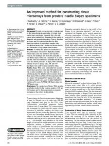
divided differences, WPCD, were utilized rather than by using the stencil [1, 7, 21, 35]/64, we expect smoother variation in divided differences at the new vertices, thus making smaller changes to the 2nd divided differences at the old vertices, the stages become: (a) Determine the divided differences at the original vertices. As before, at each old vertex compute the 2nd differences WB, WC, WD and WE (see Fig. 1)
(b) Compute new 2nd differences at the edge vertices. The stencil [1, 7, 21, 35]/64 is used to calculate the new 2nd divided differences at the new vertices.
(c) Determine the new edge vertex position For each old edge compute the new vertex position. We require that
(8)
(f)
and its z-transform can be written as
To get improvement in the continuity and precision set of the scheme (15), we adjust the shape parameter in the newly inserted vertex by using the relation . Laurent polynomial corresponding to the above mask can be written as A value of u = 0 corresponds to making no change, i.e. the scheme (7). An interesting scheme is at , where we can extract another two smoothing factors out of the mask. This can be simplified to (11)
Figure 1: Geometric rules of 4-point approximating subdivision scheme
(iii) 6-point approximating scheme We demonstrate that the 6-point scheme can be expressed by placing the new points with ratio of [1, 7, 21, 35]/64 of the 2nd divided differences of the adjacent old points. If the new
△ where
,
(16)
The improvement in the scheme (15) can be made by adding △ 6 (z) with u0 = u, n = 3 into α (z). The z-transform of the improved scheme is . (11)
3. RESULTS AND DISCUSSION To compare the different variation of the proposed scheme, we discuss continuity, precision and shape of limit curves. (i) Continuity
November-December
Sci.Int.(Lahore),28(5),5011-5015,2016
ISSN: 1013-5316; CODEN: SINTE 8
Laurent polynomial method is used to investigate the continuity of the scheme. Lemma 1. The z-transform α(z) of the scheme (7) can be written as
where
, and subdivision scheme Sα corresponding to the z-transform α(z) is C2. Proof: Suppose Sb is a scheme corresponding to the ztransform b(z) then by defining
, We find that . However by taking L = 2, it is easy to show that b[2] = {1 + 2z2 + 3z4 + 2z6 + z8}. This implies
, which show that Sb is contractive. Hence by ([10], Theorem 4.11) the scheme Sα is C2. Proofs of following lemmas are similar to the proof of above Lemma. Lemma 2. The z-transform β(z) of the scheme (10) can be written as
where
. For u = −1/4, subdivision scheme Sβ corresponding to the ztransform β(z) is C3. Lemma 3. The z-transform γ(z) of the scheme (18) can be written as
where
Sche Paramete Continui Scheme Parameter Conti me r ty nuity (10) −2 < u < C0 (18) C0 2 ......
C1
......
C1
......
C2
......
−3 < u < 3
C2
......
C3
......
−3 < u < 3
C3
...... ...... ......
−2 < u < 2 −2 < u < 2 1