An Application of Linear Programming for Block Cave Draw Control. A.R.GUEST1, G.J.VAN HOUT1, A.VON JOHANNIDES1 and L.F. SCHEEPERS2. 1 De Beers ...
An Application of Linear Programming for Block Cave Draw Control
A.R.GUEST1, G.J.VAN HOUT1, A.VON JOHANNIDES1 and L.F. SCHEEPERS2 1
2
De Beers Corporate Headquarters, Johannesburg, South-Africa Large Scale Linear Programming Solutions, Johannesburg, South-Africa
ABSTRACT: In the past various systems have been used to plan the extraction of ore from block cave operations. These systems have varied from rather sophisticated models with empirical “gravity flow” rules applied to the very rudimentary models where only the recorded mined tonnage’s have been accounted for against the available resource. The normal requirement of these models has been to only plan the movement of ground through the drawpoints. Little cognisance has been taken of the other parameters that affect the total mining operations. The intended purpose of the linear program planning system is to not only include the management, resource availability and geotechnical constraints, but to also include the mining rules. The paper will discuss the various constraints that have been considered, and attempt to illustrate where the system better serves the production system than previous ones. A brief technical discussion on the linear programming system is included.
1.
INTRODUCTION
Any attempt to operate a Block Cave operation without an effective Draw Control system would be irresponsible. Through the proper use of an effective draw system, the fragmentation within a cave can be controlled, stress build up in areas can be alleviated, and even free water within the cave can to a certain degree be directed. When De Beers introduced its first experimental cave in 1954 at Bultfontein Mine, Kimberley, a number of practical lessons were quickly learnt (Gallagher & Loftus 1960, 1961). In two instances multi-tunnel collapses occurred, resulting from stress build up within the cave as a result of incorrect draw. During subsequent years, a number of minor instances have also occurred where, through draw control oversight, drifts have come under high point loads, and have collapsed. This situation however is then only recovered by an intense adherence to a strictly controlled loading plan in adjacent drawpoints. The first draw control system which was introduced in the Kimberley Mines consisted solely of a manual recording of the daily draw records coming up from the production drifts. In the early days these records only recorded the “scraper” tally from the drifts. It was soon realised that to control the loading within a cave better, a more detailed record of where the ore was coming from was needed. This resulted in the first “winch indicator boards” being devised, and installed on the scraper winches. With this device, the winch operator was able to “calibrate” the indicator at the start of each shift, thus indicating from which drawpoint within a drift the ground was being pulled. This added to the knowledge of the draw records, and these records could then be collated with the tonnage that was then taken by the train to the ground passes. Once this data was available, and being recorded and graphically presented manually, it was then decided to use this data to proactively control the caving process. This resulted in the appointment of the first Draw Control Officer. Amongst his duties of collecting and presenting the data, was to make daily visits to the operating caves, to observe the condition
of the various areas, and to ensure that the draw control procedures were been adhered to. In the slusher drift type cave, “hang-up control” was a major problem. Not only was it a frequent problem, which is beneficial from an operational point of view, but to bring down the hang-up was also quite labour intensive. This resulted in the winch operator simply ignoring the “problem”, in order to achieve the “Call” that he was set, by readily scrapping ground from the closer drawpoints. In a typical slusher Cave at Kimberley Mines, a Cave could have up to 17 drifts cutting across the kimberlite pipe, with each drift having up to 45 drawpoints. This resulted in excess of 500 drawpoints being available (Fig. 1). With the introduction of the Draw Control system, other methods then also had to be introduced to overcome these “operational shortcomings”. This was achieved by the introduction of what became known as “strip mining”. This had the affect of splitting the Cave essentially into three separate working areas within the cave. A series of ten “open” drawpoints were separated by a series of eight to ten “closed” drawpoints. This was repeated across the width of the pipe. During any given month, a call would then be allocated to the open drawpoints. However, miners being miners, it was soon realised that the closed drawpoints, if pulled early in their “closed” period, would yield finer ground. A method to overcome this “stealing” was the introduction of a car tyre into the mouth of the drawpoint, held in place with steel chains, as well as a lead meter seal, placed by the draw control officer. Another system that was also introduced to control the “hangup” and to ensure that work was been carried out to bring the hang-up down, involved the “paint bombs”. This involved the making up of poster paint bombs on the surface. No electric light bulb was ever discarded at Kimberley Mine, as the Draw Control officer required them all for that purpose. During his routine inspections to the cave, the throwing of one of these bombs duly marked any drawpoint that was “hung-up”. The only way that the miner in charge of that section could get rid of the markings was to use explosives!
Figure 1. Plan of Wesselton Mine Block Cave Extraction Level
Having now reduced the Cave into two or three smaller sections, it became easier to ensure that the drawpoints were being worked correctly. The “closed” drawpoints were carefully monitored during the time they were out of production, to ensure that no excess point loading was taking place. The strip control had a number of benefits. Firstly it allowed the Cave to be divided into smaller sections. This allowed a meaningful call to be placed on that area. Generally, a call for eighty percent of the available drawpoints would be placed on an area. This meant that to achieve the allocated call almost all drawpoints in the section had to be worked, allowing for some drawpoints to be out of action for repairs, hang-up or just consolidating prior to any action work. The other major benefit of the strip control was fragmentation. Whilst the “closed” drawpoints were out of action, loads were being transmitted to this dead area. This resulted in secondary fragmentation of the caved material during this period. As the different Caves in the Kimberley area each had their own differing mixtures of soft and hard kimberlites, the period that a particular drawpoint could stay closed varied from cave to cave. Generally a single drawpoint could remain closed for up to six months, but some caves had to move the strip faster. This strip movement was accomplished by opening one drawpoint on one side of the strip, and closing one on the opposite side. (In caves that required faster strip movement up to two or three could be opened or closed at a time.)
The result of the work being carried out in the closed strip was evident once a drawpoint was brought back into production. Bearing in mind that this new drawpoint would have now been out of action for up to six months. For the first three weeks this drawpoint would require a high degree of secondary blasting, to get the ground to move. However, for the next few months, the ground would be well-fragmented and easy to work. 2.
EARLY COMPUTERISED DRAW CONTROL SYSTEMS
Once the main operational ‘features’ had been sorted out, and computers started to make their appearance into industry, the first computerised Draw Control System was written and introduced into Kimberley Mines, in 1967. The system basically followed what the manual system had been doing, but obviously allowed for a more efficient data handling, and graphical output. A specific feature of the system was the introduction of a “Control Horizon”. This in affect restricted the available tonnage to some defined percentage of the total reserves allocated to the drawpoints. The benefit of this was an attempt to control the cave by not allowing the draw of any drawpoint to get excessively out of control. No call would be allocated to any drawpoint that had exceeded the Control Horizon.
System Flow
The system calculated the calls for each drawpoint on an inverse weighting allocation, based on the number of months left to deplete the reserves, at the previously calculated average tonnage per month.
VMS Tracking data from drawpoint to plant
Within the system data on Area Call, maximum production per drift, average production per drawpoint, maximum production per drawpoint, working drawpoints required were all required prior to setting up calls. The system would then ensure that none of these criteria were violated. The system would iterate the allocated calls until a solution was achieved, or an error message would be generated suggesting some remedial action. This type of message would become common on nearing the Control Horizon, and would indicate a lifting of the Control Horizon. No attempt was made to introduce sophisticated gravity flow rules into the draw, as the maximum tonnage extracted per drawpoint per day rarely exceeded thirty. With the advent of the personal computer, graphical presentations became a lot easier to generate. Also user interaction with the computer program was possible, and the very first version of Gemcom’s PCBC was written and introduced onto Premier Mine (Owen & Guest 1994). This for the first time introduced Laubscher’s empirical gravity flow rules into the draw control system (Laubscher 1994). One of the major shortcomings of this system, was the lack of production based input into the setting of calls. This system was run from a Draw Control base only. It was only in its latter years, when Production/Draw Control meetings were introduced on the mines, that some degree of “production constraints” were introduced. These were then accounted for in the system during the allocation of the drawpoint weightings. With the introduction of a draw control system based on linear programming, it is anticipated that by including and integrating constraints from other disciplines like geology, mining and metallurgy into the system it will become more accepted as a business planning tool and not perceived solely as a policeman. This has been done by not only accommodating for drift and drawpoint constraints, but also Load-Haul-Dump equipment, ore pass, transfer level, train, as well as crusher availability into the allocation of calls. 3
BRIEF DESCRIPTION OF A COMPLETE DRAW CONTROL SYSTEM
A successful and complete Draw Control System in a cave mining operation not only consists of a long term scheduling tool, the linear programming. Other components to be integrated into the system are an accurate data collection system, an appropriate cave simulator, a correct mineral resource database and a short term scheduling system. Figure 2 shows a simplified system flow through these different components making up the Draw Control System as envisaged by the authors. It is not within the scope of this paper to describe in detail all components within the draw control system. This will be covered in a future paper.
Description Actual production and other relevant node data as measured by a Vehicle Monitoring System. This data can be obtained per shift or by accumulated time periods.
Determine resource movements
Query of VMS data to summarise all the movements from a source (e.g. drawpoint) to destination (e.g. ore pass) per shift or accumulated time period.
Drawbell interaction and interface mixing
Apply the drawbell interaction and interfacing mixing algorithm to simulate the caving process. Sequence is important in this process.
Mineral Resource Database (MINRAS)
After the drawbell interaction and interface mixing the resource must be updated, so that Linear Program Draw Control System uses the latest updated resource.
LP long term scheduler on the updated resource model
Linear Program based long term scheduler to run once the resource is updated and the constraint set has been modified and checked.
short term scheduler new call based on planned (LP) tons and actual (VMS) tons mined
Production within total ore flow
Short term scheduler to guide production in achieving long term plan as produced by long term scheduler
Short term production call according to a Linear Program based long term scheduler plan.
Figure 2. A complete Draw Control System flow chart.
4.
INTRODUCTION INTO LINEAR PROGRAMMING BASED SYSTEMS
The search for the best, the maximum, the minimum, or, in general, the optimum solution to a variety of problems has entertained and intrigued man throughout the ages. Obviously, by doing so companies are moving into a more efficient production scenario, based on sound mathematical principals, and for which benefits have been clearly stated. Since the problem of linear programming was first developed and applied in 1947 by George B. Danzig, Marshall Wood and others in the US and UK military, applications have been extended in virtually all areas of the economy, including many areas in the mining industry.
The optimisation of a linear function subject to linear constraints is simple in mathematical structure but powerful in its adaptability to a wide range of applications. The mathematical technique of Linear Programming is a search routine where the utility to be optimised is expressed as a linear equation and the domain in which the search takes place, is confined by boundary or constraint linear equations.
Workstations on local LAN and connected to SQL-Server
In the case of non-linear utilities or constraints, an extension of Linear Programming, Mixed Integer Programming, is fruitfully used for formulation purposes. The same applies to “GO – NO – GO” modelling. Mixed Integer Programming is extensively used in the Draw Control System. Generally, Mixed Integer Programming models require more computing resources than Linear Programming models. Modern day Linear Programming and Mixed Integer Programming models of real world large mining and metallurgical complexes can have matrix dimensions of up to hundreds of thousands of variables in as many constraints and in order to solve these models, a mature matrix generator, OMNI and optimiser, CPLEX are required. By using mature software, management can be sure that the planning integrity is beyond doubt due to superior data to matrix conversion methodologies and optimisation techniques employed. Tabulated below is an indication of the speed and size of problems that successfully have been solved with Linear and Mixed Integer Programming. Operation
No. of constraints
Variables
Integers
Solving time
Alluvial LOM Front Cave
34284
35785
5417
6.5hrs
4649
4683
1176
110 sec
Open Pit
11141
9002
3030
1.5 hrs
Marine mining
16754
13362
4416
30 sec
Table 1. Examples of Linear and Mixed Integer Program matrices and solution times. These performance figures are the output from a Silicon Graphics Origin 200, with 256MB of RAM, 4 x R10000 Mips processors. Currently a Client-Server systems approach is adopted in an attempt to minimise the cost of implementing expensive matrix generation and optimisation software at the sites. This however is one approach, and each site could actually have individual set-ups. Figure 3 illustrates a typical configuration for a Draw Control / Production Planning System of an operating environment at De Beers sites.
Operations environment (remote) Draw control and planning workstations. Clients running front and back-end applications linking to a RDBMS.
Servers on local LAN - CHQ WAN
WAN or Internet
CHQ environment (centralised)
Transfer of relevant data to be optimised on servers
Server environment running matrix generation (on NT platform) and optimisation (on Unix® platform).
CHQ : Corporate Head Quarters LAN : Local Area Network WAN : Wide Area Network SQL : Structure Query Language RDBMS : Relational Database Management System
Figure 3. A typical operating environment for Draw Control or Production Planning System at De Beers sites.
5
PRODUCTION PLANNING SYSTEMS BASED ON LINEAR PROGRAMMING
Before elaborating on the Draw Control System, it may be worthwhile looking at other Production Planning Systems based on Linear and Mixed Integer Programming. Linear Programming based principles have successfully been used for the Life Of Mine and shorter term scheduling in open pit and strip mining environments, each with their own specific needs (Hoerger et all 1999, Graham-Taylor 1992, Scheepers & Wellbeloved 1992) Life of Mine and short term planning systems based on Linear / Mixed Integer Programming have been developed since 1974 for strip mining operations, for the following reasons: • • • • •
World-class deposits had to be mined responsibly under legal constraints. The need to split large areas into manageable portions where each sub-area constitutes a mine with its own treatment facility. Sub-areas are split into many mining blocks, which carry relevant parameters for planning efficiencies, economic and sustainable depletion strategies. For many models like grade, size, density, revenue, costs and contribution there can be large variability from block to block. Ore blending constraints are required to maximise plantoperating efficiencies.
A typical Life of Mine Linear Programming model for strip mining operations would include the following: •
•
• • •
An Objective function which maximises the total contribution at various levels of costing like direct mining and treatment, direct mining and treatment and overheads etc. The Planning is broken up into multi-time periods, which are user definable. It must be emphasised that the optimisation is not done individually for each time period but for all time periods simultaneously. In this way the optimisation is seen over the Life of Mine, as well as adhering to the constraints and calls of each individual time period. There is provision for multi-production areas (mines and treatment), each carrying its own set of constraints and calls. Optimisation can be done on the total resource or parts thereof A set of constraints, consisting of an upper and lower limit for each parameter, per period, per production area. It can be summarised as : Mining: Percentage Cubic metres per block to allow for specific amounts or the total block itself ♦ Allow for a certain percentage of stripped reserves in an area or sub-area so that flexibility of mining ore due to short-term production problems can be achieved. ♦ Allow for a minimum amount of ore to be left behind in a block to avoid the problem of having a multitude of remnants. ♦ Allow for certain amount of ore and overburden to cater for various vehicle requirements and capacities. ♦ Allowance for certain ton-kilometers to avoid taking only material in close proximity to treatment plants. ♦ Waste tonnage range to cater for the stripping fleet. ♦ Ore tonnage range to cater for a particular mining fleet. ♦ Machine hours on all major production equipment. ♦ Allow for blocks to be mined in sequence to cater for dragline deployment and logistics. ♦ Fix certain blocks to be mined to overcome practical problems like laying pipelines. ♦ Allow for mining precedence per block to cater for different waste and ore horizons. Plant: ♦ Allowance for certain volume (tons or cubic metres) per processing plant. ♦ Blending of different rock types agreeable to plant efficiency. ♦ Allowable percentages of clay, wet, dry, soft, hard or cemented material. Economic: ♦ Escalation or de-escalation of various levels of costing per block. ♦ Revenue escalation or de-escalation per block ♦ Contribution limits by looking at the difference between revenue and cost. ♦ Variable discount factor per period ♦ Required Profit to Revenue ratio per area or subarea. ♦ Exchange rate per period.
General: ♦ Allowance for a grade (carats per cubic metre or carats per hundred ton) range. ♦ Allowance for a particular size range. ♦ Allowance for a number of carats. ♦ Allowance for a number of stones. ♦ Allowance for a density range. •
User friendly front and back-end database systems are written around the Linear / Mixed Integer Programming component, allowing the mine planner flexibility and power to mix and match multiple planning resources to multiple planning scenarios.
6
THE LINEAR PROGRAMMING COMPONENT OF THE DRAW CONTROL SYSTEMS
As illustrated in the draw control system flow chart (Fig. 2), the long-term scheduler based on Linear Programming is not the only, but nevertheless an important and essential component of a successful Draw Control System. The basic actions within this specific component are shown in figure 4. Official Mineral Resource Database
Select planning resource Establish planning scenario Submit scenario to be optimised Create matrix file
Planning Mineral Resource Database
Optimise matrix file Analyse results
Figure 4. Iterative process within the Linear Programming based long term scheduler. During the initial examination into the use of Linear / Mixed Integer Programming techniques to solve for an optimum depletion strategy of a block cave it soon became apparent that the geotechnical rules and constraints would form the major and overriding control. These rules would limit areas of flexibility, as one cannot select material to be mined from columns without adhering to strict sequencing and relationship criteria between adjacent columns. Kimberlite ore bodies are variable in nature and large variation in grade can occur within the pipe, which makes mining to a constant grade difficult and even more so if geotechnical rules are adhered to which will limit areas for accessibility. However it was felt that besides the all-encompassing geotechnical constraints it was still necessary to model the entire cycle of ore extraction and ore processing and would thus also include maxima and minima constraints, per period, for the following:
1.
2. 3. 4.
Ore flow process, which will highlight the material that can pass from node to node. The nodes that have been modeled are tunnels, ore passes, haulage systems, underground accumulation areas, shaft systems and treatment plant. Metallurgical constraints that will include plant capacities and rock type blends. Economic constraints that will include cost and price escalation or de-escalation, discounting, exchange rates and Profit to Revenue ratio ratios. Geological constraints like grade, carats, stones, size and density.
By using the combined constraint set it is possible to produce a better or optimised production mix resulting in better utilisation and efficiency of production resources, even though only small areas of flexibility exist because of the strict geotechnical rules and constraints. A breakdown of the important aspects of the Linear and Mixed Integer Programming method and formulation for Draw Control Systems is discussed below. 6.1
Objective Function
The objective function for the Linear and Mixed Integer Program Draw Control System will be to maximise the NPV over Life of Mine and within each of the user defined multitime periods. The maximisation of NPV is closely associated with maximising ore tons, as the ore tons generate revenue. The model should thus minimise the mining of waste tons as they do not generate or contribute towards revenue. This ensures that the Linear / Mixed Integer Program not only achieves the best ore tonnage model but the best ore tonnage model at the best profit. With the use of discounting factors in the user defined periods the model will always want to mine to a maximum earlier rather than later, as this will optimise the NPV as stated by the objective function. 6.2
Other resource data The Linear Programming based long-term scheduler is also capable of incorporating the treatment of other resources such as sublevel cave blocks. If included into the program, input from these resources should be the same as for stockpiles and dumps. 6.3 Constraints The Linear Programming scheme allows constraints to be set in terms of a minimum and maximum limit on any output per multi-time period. Setting these upper and lower bound requirements needs careful attention and should be subject to properly designed procedures, audited by consultants from the relevant disciplines. Three major groups of constraints will be discussed in the following sections. The first group is derived by strict geotechnical rules imposed on the optimal solution. The next group of constraints is dictated by mining limitations. The last set of constraints includes straightforward requirements prescribed by metallurgical requests. Geotechnical constraints •
COLUMN DRAW RATES The Linear Programming application caters for a limited draw rate for each column within each time horizon. The column draw rates in the current Linear Programming versions are expressed as tons per period.
•
PRECEDENCE OF ACCUMULATED TONS DRAWN A set of constraints is activated, which stipulates, that, a given column can only be drawn from, once a user defined tonnage has been drawn from its predecessors. Put differently, drawing from a column is permitted, only if the accumulated ton drawn from its predecessor adheres to a pre-specified minimum. This formulation generates one integer variable per column and its predecessor.
•
LIMITS IN DIFFERENCES OF ACCUMULATED TONS DRAWN BETWEEN COLUMNS WITHIN TIME HORIZONS The model is constrained by a set of equations to ensure that the accumulated tons drawn from a column will be within a pre–specified range of accumulated tons of neighbouring columns.
Resource input data
Vertical resource columns The cave orebody is split up in vertical resource columns, positioned above the drawpoints. The required input data for these resource columns can be summarised as follows: • • • • •
Opening resource in terms of ore tons at the start of the planning horizon. Estimate of the ore to waste mix in terms of a percentage value. Historical accumulated tons drawn per column. Historical kimberlite tons drawn per column. Upper and lower capacity flow rates in terms of tons of ore per period.
It is up to the geology and survey department to ensure that the draw control officer running the Linear Programming application has the correct data available at all times. Stockpiles and dumps on surface Ore from resources on surface, e.g. stockpiles and dumps can be activated by the user to blend in with the ore streams from the draw points to the plant. Both resource types contain opening volume (tons or cubic meters), percentage kimberlite, percentage waste, grade, density, stones, percentage concentrate, percentage rocktype(s).
A further relationship is generated to nullify the constraint, once one of the columns has been depleted. This set of constraints is dependent on its input from the rock mechanics and mine stability experts in order to limit the development of “rat-holing”. •
LIMITS IN RATIOS OF TONS DRAWN BETWEEN COLUMNS WITHIN TIME HORIZONS The model is constrained by a set of equations to ensure that the tons drawn from a column, will be in a user specified ratio of tons drawn from neighbouring columns. A further relationship is generated to nullify the constraint, once one of the columns has been depleted. This formulation generates two integer variables per predecessor draw point. This set of constraints is dependent on its input from the rock mechanics and mine stability experts in order to ensure a steady and acceptable angle within the cave back.
Mining constraints •
ORE FLOW CONSTRAINTS The system has the ability to define any number of relevant ore flow processes and the associated capacity of these routes. The ore flow currently caters for: • Tunnels for the accumulated material from the drawpoints. • Ore passes for accumulated material from various tunnels. • Haulage for the accumulated material from ore passes. • Underground accumulation areas store material from various haulage routes. • Shaft systems for accumulated material from various underground accumulation areas.
Currently two implementations of this interface are in various stages of commissioning and testing, one for a Front Cave, the other for a Panel Cave operation. When the user opens the front and back-end program a logon screen similar to Figure 5 appears.
The user has control over the minimum and maximum flow capacities of each ore flow route within each time horizon. Metallurgical constraints •
TREATMENT PLANT The plant treating the ore produced from the cave or transported from the other resources can be included in the optimisation calculation. The required input for the plant is: upper and lower throughput capacities in terms of tons ore per period. Tolerated minimum and maximum ore to waste ratio in the plantfeed expressed as a percentage. The plant is defined as an ore process unit with an upper and lower throughput capacity. All ore streams from the draw points via the haulage routes combined with the ore streams from the surface resources are directed to the plant. The user has control over the maximum and minimum kimberlite to waste ratios in the ore stream routed to the plant, i.e. drawn from all the active draw points and drawn from surface resources. This control is available per time horizon.
Economic constraints
Figure 5. Opening screen when logging onto the draw control system. The front-end program is able to cater for different levels of users and has an auditing facility to log any changes made during a session. Depending on the user profile, the program will assign specific rights to the user. A draw control officer for instance will only be allowed to run the simulations, whilst the Geotechnical Engineer may change any of the critical parameters. If an authorised user changes crucial rules in the system, an audit table is created and the user is prompted to give a justification why these changes were made. This information and the user name are stored in the audit table, along with all changes made. When the user opens a working scenario in the system, a screen similar to Figure 6 appears.
Escalation or de-escalation of various levels of costing per block to take into account the perceived cost for each time period. Likewise for revenue, each period can be adjusted for a price increase or decrease. Associated with each time period is a discount factor use to estimate the present value of money for that particular time period. Further economic constraints are the required profit to revenue ratio and exchange rates to be used per time period. Geological constraints Geological constraints like grade; carats, stones, size and density can be used per time period and can be useful in overall scenario planning.
7
INTERFACE BETWEEN USER AND LINEAR PROGRAM INPUT
Due to the complexity of Linear program input requirements a user-friendly front and back-end program was written to facilitate the creation of the matrix. This interfaces with OMNI (matrix generator).
Figure 6. General information associated with a typical simulation scenario. Apart from the title, project name, date, name of the creator and the comments the user may add, essential information required here is which resource (Fig. 3) has been used and
what accumulated mined data has to be loaded from the Vehicle Monitoring System. When the user selects on the next tab in the scenario window, a screen similar to Figure 7 appears.
Figure 8. Production calls per period. As can be seen, the metallurgical constraints are not only put in as a maximum limit to its capacity in tons but it also allows a certain percentage waste of the total production mixture.
Figure 7. Period definition, drawpoint status and planned draw rates for a scenario.
When the user clicks the ‘constraints’ tab, a screen similar to Figure 9 appears.
As the Linear Program uses multi time horizons and optimises over the all periods, the user needs to define the number of periods by adding a period number, a description and how many days are within that period. The user also has to set the minimum and maximum draw rates, the status of the drawpoint (open or closed) for each drawpoint, for each period. Vast experience and data from existing or ceased cave mines allow De Beers personnel to assess what draw rates are acceptable at the operation for which the Draw Control System is devised. At Premier Mine, maturity rules are in place to forecast at what rate the drawpoints can produce, depending on the drawpoint maturity (Bartlett 1998). The maturity of a drawpoint is expressed in terms of months in production or tons produced from that drawpoint, whatever the lowest value. At Koffiefontein Mine, the column draw rate is expressed in millimetres draw down per day. As the column draw rates in the Linear Programming are required in terms of tons per period the front to back end program must convert the user input in terms of millimetres per day to tons per period. A default maximum draw rate value is assigned to all drawpoints during all multi-time periods. The user may change these default values but these may not exceed a limit value kept in a secure database. All users have read access to this database but only a few authorised users may change these values. This ensures that the system cannot be abused, on purpose or by accident and management can at all times verify who made the changes and what justifications were given. When the user selects the ‘calls’ tab, a screen similar to figure 8 appears. Here the user decides what the total production call is per period that will be treated by the plant and how this is split between the different resources.
Figure 9. The constraints table in the front to back end program. For each period, a generic set of constraints is applied in terms of geotechnical and mining related parameters. Mining constraints could dictate that the accumulated mined profile in a certain section should have an overall slope angle of twenty-five degrees. This angle ensures that there is enough time to construct and open new drawpoints without obstructing the global production. Another constraint could be that there is a relation between two neighbouring drawpoints depleting the same ore column. The ratio between the production of the top drawpoint and the production of the bottom drawpoint could be designed at forty to sixty (equals sixty six percent). The user supplies the information in specified units (degrees or ratio’s or tons) and the front end will translate these into tons, as required by the Linear Programming (see section 6.4).
Exceptions to the general applied rules may be defined in a separate window (see ‘Matrix Constraints’ button in Figure 9). The variance between planned and actual production should be kept within acceptable limits as determined by the constraints discussed in section 6.4 and illustrated in Figure 9. However, if the actual production is in far excess of what was planned by the long term scheduler, some of the rules may have to be violated to ensure that the system finds a solution for the next long term plan and rectifies the overall situation. The strength of the Draw Control System described here is the ability to provide a solution (by adjusting the rules), even if the production is completely off track as what was planned by the Linear Programming application. 9
CONCLUSIONS
The major benefits of the Linear / Mixed Integer Programming system to previous systems have been established:1) Draw control is now an integral part of the overall business cycle, which includes technical input from geology, mining, metallurgy and finance. 2) The Linear and Mixed Integer Programming approach optimises over Life of Mine as well as multi-time periods within Life of Mine. In this way the model is always aware of the long term implications as well as solving short-term constraints. e.g., Linear Programming is used to decide when it is the best time to start support works in certain tunnels. This is only possible since an optimisation is done over a multi time period. 3) Fast turn around time regarding output, which means that many options, can be run and analysed, giving the planner and management flexibility regarding different options and confidence in the outcomes. 4) All actual production data (history) is stored allowing a re-depletion and re-planning phase to take place, which can be compared to the current or other depletion strategies When comparing Linear and Mixed Integer Programming results to manual spreadsheet type systems there have been up to 20% improvements. 5) Ability to store the desired plan with its constraint set, making the management, control and auditing task feasible. 6) The system is flexible and generic, allowing for many different planning scenarios and the ability to pick and choose from different resource combinations. 7) For feasible outcomes one always knows that the optimum result for a given constraint set is being presented. 8) With the advent of new technology (hardware and software) and the incorporation of new mathematical algorithms (e.g. Gomory cutting plane integer algorithm), the run time of Linear Programming based systems is decreasing rapidly. 11
ACKNOWLEDGEMENTS
The permission of the Director, Operations, De Beers Consolidated Mines Limited, to present this paper is gratefully acknowledged. The authors acknowledge the work of Mr. A. Langbridge and his team at Technical Systems, De Beers Consolidated Mines Limited for the successful development and implementation of the front-end program. Gratitude is expressed towards Mrs. C.F. Bruwer of L.S.L.P.S. for coding the matrix generator.
12
REFERENCES
BARTLETT, P.J., 1998. Unpublished internal report. Premier Mine, De Beers Consolidated Mines. CPLEX 6.60 2000. Registered trademark of ILOG, Paris, France. GALLAGHER, W.S. & LOFTUS, W.K.B. 1960. Block caving practice in De Beers Consolidated Mines Limited. Mine Managers Association of South Africa, Papers and Discussions. GALLAGHER, W.S. & LOFTUS, W.K.B. 1961. Yielding arches for support of block cave scraper drifts. Ibid. Mine Managers Association of South Africa, Papers and Discussions: pp439 – 458. PCBC 2000. GEMCOM Software International Inc., Vancouver Canada. GRAHAM-TAYLOR T. 1992. Production Scheduling using Linear and Integer Programming, AusIMM Annual Conf., State of the art – a product of 100 years of learning: 17-21, Broken Hill, NSW, Parkville, Vic., Australia. HOERGER S., BACHMANN J., CRISS K., SHORTRIDGE E.. 1999 Long term mine and process scheduling at Newmont’s Nevada operations. APCOM 28th Symposium at the Colorado School of Mines: Computer Aplications and Operations Research to the Mining industry. LAUBSCHER, D.H. 1994. Cave mining, the state of the art. Journal of the South African Institute of Mining and Metallurgy. October 94: 279-293. OMNI 2.52 2000. Registered Trademark of Haverly Systems Inc., Denville, USA. OWEN, K. C. & GUEST, A. R. 1994. Underground mining of kimberlite pipes. XVth Congress, Johannesburg, SAIMM, vol. 1, pp207-218 PEELE, R. 1941. Practice at De Beers Diamond Mine, Kimberley, South Africa. Parkinson, L. and Dickson, H.T.(eds.) 3rd Edition, Chap 10, pp 392 – 398 SCHEEPERS L., WELLBELOVED D., 1992.Optimisation of Integrated Mining and Metallurgical Complexes by means of Linear Programming and Case Study. Survival Strategies for the Metallurgical Industry ,Johannesburg, South Africa SAIMM. WAGNER, P.A. 1914. The diamond fields of Southern Africa. Struik, Johannesburg. WILLIAMS, G. 1902. The diamond mines of South Africa – some account of their rise and development.