846
IEEE TRANSACTIONS ON AUTOMATION SCIENCE AND ENGINEERING, VOL. 8, NO. 4, OCTOBER 2011
Linear Programming SVM-ARMA2K With Application in Engine System Identification Zhao Lu, Member, IEEE, Jing Sun, Fellow, IEEE, and Kenneth Butts, Member, IEEE
Abstract—As an emerging non-parametric modeling technique, the methodology of support vector regression blazed a new trail in identifying complex nonlinear systems with superior generalization capability and sparsity. Nevertheless, the conventional quadratic programming support vector regression can easily lead to representation redundancy and expensive computational cost. In this paper, by using the 1 norm minimization and taking account of the different characteristics of autoregression (AR) and the moving average (MA), an innovative nonlinear dynamical system identification approach, linear programming SVM-ARMA2K , is developed to enhance flexibility and secure model sparsity in identifying nonlinear dynamical systems. To demonstrate the potential and practicality of the proposed approach, the proposed strategy is applied to identify a representative dynamical engine model. Note to Practitioners—The identification of complex nonlinear engine systems poses challenges on the efficiency, flexibility and generalization capability of the identification algorithms. Inspired by the triumphs of support vector learning methodology in pattern recognition and regression analysis, an innovational nonlinear systems identification algorithm, LP-SVM-ARMA2K was developed in this paper as a significant stride toward the fusion of modern machine learning essentials into practical identification strategy for industrial systems. In particular, the possible generalization of LP-SVM-ARMA2K via more complex composite kernel functions is also discussed to meet the diversity of industrial practice. Index Terms—Composite kernel, generalization, linear programming, model sparsity, nonlinear system identification, support vector regression.
I. INTRODUCTION S THE TURNING POINT in the history of machine learning methods, the development of kernel-based learning systems in the mid-1990s comes with a new level of generalization performance, theoretical rigor, and computational efficiency [1], [2]. The fundamental step of the kernel approach is to embed the data into a Euclidean space where they interact only through inner product and the patterns can
A
Manuscript received July 30, 2010; revised November 07, 2010 and February 22, 2011; accepted March 21, 2011. Date of publication April 25, 2011; date of current version October 05, 2011. This paper was recommended for publication by Associate Editor S. Bogdan and Editor M. Zhou upon evaluation of the reviewers’ comments. Z. Lu is with the Department of Electrical Engineering, Tuskegee University, Tuskegee, AL 36088 USA (e-mail:
[email protected]). J. Sun is with the Department of Naval Architecture and Marine Engineering, University of Michigan, Ann Arbor, MI 48109 USA (e-mail: jingsun@umich. edu). K. Butts is with Toyota Motor Engineering and Manufacturing North America, Inc., Ann Arbor, MI 48105 USA (e-mail:
[email protected]. com). Digital Object Identifier 10.1109/TASE.2011.2140105
be discovered as linear relations, thereby reducing many complex nonlinear problems to tractable linear problems [3], [4]. As is typical of non-parametric kernel learning systems, the support vector machine (SVM) has been successfully applied in nonlinear regression by introducing the –insensitive loss function [3], [5]. With the aid of duality, the conventional support vector regression is formulated as a convex quadratic programming (QP) problem, through which a sparse model can be obtained with generalization capability. Recently, the quadratic programming support vector regression (QP-SVR) have been successfully applied in identifying the nonlinear dynamical systems [6]–[8], which can be traced back to the use of Green functions and generalized Fock space for nonlinear systems identification in earlier research work [9], [10]. However, since all data points not inside the -tube are selected as support vectors, redundant data points appear in the non-parametric model representation derived from quadratic programming support vector regression (QP-SVR) when used for identifying complex nonlinear dynamical systems. This results in the onerous computational task, and also violates the principle of Occam’s razor, which argues that the model should be no more complex than is required to capture the underlying system dynamics. Instead of enforcing flatness in feature space as is the case with QP-SVR, the linear programming support vector regression (LP-SVR) employs the norm as regularizer, which inherently enforces sparseness of the solution. This leads to the superiority of LP-SVR in model sparsity, flexibility in using more general kernel functions, and computational efficiency [11], [12]. Albeit the norm has been introduced in support vector classification for various purposes [13]–[15], until very recently a few LP-SVR algorithms were developed for modeling nonlinear dynamical systems from input–output data, and simulation studies have demonstrated the potential of LP-SVR in the realm of nonlinear systems identification [16], [17], [19]. In this paper, inspired by the challenge of providing effective engine models to support control strategy development and system integration, we aim at developing advanced identification algorithms for modeling dynamical system output as a nonlinear function of the past system inputs (moving average) and past system output (autoregression). On the strength of LP-SVR and the algorithm of SVM-ARMA proposed in [21], we develop a novel nonlinear identification approach, LP-SVM-ARMA , and investigate its implications on model generalization and complexity. The issue of engine modeling has been widely studied by the industrial and academic engine control community, and many
1545-5955/$26.00 © 2011 IEEE
LU et al.: LINEAR PROGRAMMING SVM-ARMA
WITH APPLICATION IN ENGINE SYSTEM IDENTIFICATION
different types of models with different levels of complexity and fidelity can be found in the literature [18]–[20]. Existing engine models that serve to support engine control and calibration are often phenomenological in nature and they generally can be categorized into two classes: the gray-box models where certain first principles are combined with system identification techniques in the modeling process, and the black-box models which rely primarily on data and regression techniques for model development. While the thermodynamic process associated with engine operation has many statistical characteristics and empirical engine mapping is a common practice, the engine modeling has been rarely attacked from the angle of non-parametric statistical learning. Hence, our research presented in this paper also sheds light on non-parametric statistical modeling for engine systems. The following generic notations will be used throughout this refer to scalar paper: non-boldface symbols such as valued objects, lower case boldface symbols such as refer to vector valued objects, and finally capital boldface symbols such as , will be used for matrices.
847
autoregression (AR) and moving average (MA). This is quite different from the regressor used for general function approximation problems and, in particular, AR and MA may affect the output of the dynamical system differently. This is the motivation for using the composite kernel in the context of LP-SVM, which leads to a new powerful tool, LP-SVM-ARMA , for nonlinear dynamical system identification. With the capability of characterizing the roles of AR and MA by different kernel functions, the LP-SVM-ARMA provides more flexibility in representing nonlinear dynamical systems and underpins advanced analysis. In [21], the composite kernel has been used for the QP-SVR in identifying the nonlinear dynamical systems, where the primal regression problem needs to be converted into its dual for being cast in terms of the kernel functions. In [22], the least square SVM with composite kernel is adopted to predict chaotic time series, where the main problem is the loss of sparsity. In this research, the simulation experiments on an inline four cylinder engine system are conducted to evaluate the utility of the proposed algorithm, and the results provide compelling evidence and a basis for optimism.
II. MOTIVATION AND INNOVATION Conventionally, the problem of system identification consists of setting up a suitably parameterized identification model and adjusting the parameters of the model to optimize a performance function based on the error between the system to be modeled and the identification model outputs. Contrary to that, the identification model obtained by support vector regression is non-parametric and represented as the kernel expansion on the support vectors, which are the data points in a selected subset of the training data [4], [5]. As an important member in the family of kernel methods, the SVM is a universal approach for estimating the multidimensional function per se. It has been gaining popularity in the field of pattern recognition and nonlinear regression. On the other hand, due to the fact that SVM represents the model as a kernel expansion on the support vectors, the model sparsity, which is defined as the ratio of the number of SVs to the number of all training data points, is the key to alleviate redundancy and control model complexity. Pursuant to Occam’s razor principle, also known as the parsimonious principle, which ensures the simplest possible model that explains the data, low sparsity is closely related to model generalization and nonlinear model building. Otherwise, the size of a nonlinear model can easily become explosively large, which usually results in the degradation of the generalization capability. In an attempt to secure the succinct model with less computational effort, the LP-SVR capitalizes on the norm of the coefficients vector in the kernel expansion as a regularization term for controlling the model complexity and structural risk. Most of the earlier works in applying support vector learning to nonlinear systems identification [6], [7], [16], [17] treat the issue of systems identification as a general regression problem. However, in the scenario of nonlinear dynamical systems identification, the regressor used for identifying the NARX (Nonlinear AutoRegressive eXogenous) model consists of two parts:
III. LP-SVM-ARMA Consider a nonlinear dynamical system with inputs and single output , at the time instant the states of the discrete-time processes of the output and multiple inputs are denoted by the vectors and , where , . Hence, is the vector concatenation of the output and , and input states at that instant. It is assumed that the dimension of the vectors and , respectively, are large enough so that the predictable part of the process is completely captured. To identify the nonlinear dynamical systems described by (1) most of the existing approaches employ the regression vector , in which the NARX model is considered in a wide and implicit sense. However, the necessity and possible benefit brought has been recognized in by partitioning the regression vector [23] and [24]. In [23], only the partially linear model was discussed and the least square SVM used there may lead to the loss of sparsity. Instead of stacking the AR and MA components together into the regressor , SVM-ARMA admits the following model for dynamical systems identification [21]:
(2) where and are the kernel functions for the autoregresand moving-average part , respectively, and sion part is the number of available samples. The summation in (2) is called the composite kernel [25], which can be
848
IEEE TRANSACTIONS ON AUTOMATION SCIENCE AND ENGINEERING, VOL. 8, NO. 4, OCTOBER 2011
viewed as the induced inner product in the direct sum of two different Hilbert spaces [21]. As soon as the kernel functions and are specified for characterizing the behavior of AR and MA, the model can be built by estimating the coefficients . As a non-parametric model, the vector SVM-ARMA represents the model in the form of composite kernel expansion on all of the training data. Hence, the number of nonzero components in the coefficients vector largely determines the complexity of the kernel expansion model. Herein, in an attempt to control the complexity of the model representation and thereby secure excellent generalization performance [26], norm of the coefficients vector of the composite kernel the expansion is employed as the regularization term in the objective function to be minimized, which stems from the approximation for the norm and usually leads to the small cardinality of the support vector subset. In this way, the non-parametric model (2) can be synthesized by solving the following regularization problem:
kernel are in the class of translation-invariant kernels, and the polynomial kernel and sigmoid kernel are examples of rotation invariant kernels. In fact, every kernel function has its specific feature in measuring the similarity of the different patterns, and the use of kernel functions makes it possible to deal with complex nonlinear relations. To guarantee the positive definiteness of the Hessian matrix, only the Mercer kernel can be used in QP-SVR. However, the linear programming problem is still solvable with a symmetric non-Mercer kernel in LP-SVR [16]. and , the regularizaBy introducing the slack variables tion problem (3) can be equivalently transformed into the following constrained optimization problem:
(3)
(10)
where the parameter controls the extent to which the regularis defined as the ization term influences the solution and –insensitive loss function (4) where is the error tolerance. Geometrically, the -insensitive loss function defines an -tube. The vector pairs in model representation (2) corresponding to the nonzero coefficients are defined as support vectors in SVM-ARMA . Several widely used kernel functions are available for constructing the composite kernels. Gaussian radial basis function (GRBF) kernel
where the constant determines the tradeoff between the sparsity of the model and the amount to which deviations larger than can be tolerated. From the geometric perspective, it can be followed that in SV regression. Therefore, it is in the constrained sufficient to just introduce slack variable optimization problem (10). Thus, we arrive at the following formulation of SV regression with fewer slack variables:
(5) Polynomial kernel (6)
(11)
Sigmoid kernel (7) Inverse multi-quadric kernel (8) Exponential radial basis function kernel
In other words, the calculation of the expansion coefficients vector and the selection of the support vectors in (2) can be accomplished by solving the optimization problem (11). For the purpose of converting the optimization problem above into a linear programming problem, the components of the coeffiare decomposed as cient vector and their absolute values follows:
(9)
(12)
where are the adjustable parameters of the above kernel functions. The RBF kernels and inverse multi-quadric
. Apparently, the decompositions in (12) where are unique, i.e., for a given there is only one pair
LU et al.: LINEAR PROGRAMMING SVM-ARMA
WITH APPLICATION IN ENGINE SYSTEM IDENTIFICATION
fulfilling both equations. It is underscored that both variables . In this cannot be positive at the same time, i.e., way, the optimization problem (11) can be written as
849
us more flexibility to use different kernels for characterizing the different inputs when necessary, i.e.,
(17)
(13)
Next, define the vector (14)
and express the
norm of
as (15)
with the
-dimensional vector and , the optimization problem (13) can be formulated as the linear programming problem as follows:
where is the generalized composite kernel. In [21] and [25], to accommodate the possible coupling between systems input and output of a single-input nonlinear dynamic system, the algorithm of SVM-ARMA was developed, where the cross-kernel was introduced to extract the cross information from the data. However, for multi-input nonlinear dynamic systems, the coupling may exist amid all system inputs and output. For simplicity, it is postulated that and output have the same the inputs , dimension here. Otherwise, some amount of redundant information can be added to achieve the uniformity of dimensions [21]. Evidently, the introduction of cross-kernels into the generaland/or ized composite kernel, such as cross-kernels , , , may easily result in the complication of model representation and difficulty in choosing appropriate kernel functions. A potential solution to this problem is to map the system inputs and output into mutually orthogonal Hilbert subspaces, which makes the cross-kernels vanish because the inner product between vectors belonging to mutually orthogonal Hilbert subspaces is zero [28]. This also makes it possible to conceptualize the nonlinear decoupling identification for nonlinear multi-input dynamic systems in the framework of kernel learning. The in-depth study on this issue will be left as further work. IV. APPLICATION OF LP-SVM-ARMA TO ENGINE MODELING
(16)
, and where is an identity matrix. The and are the kernel , matrices with entries defined as , which act as the interface between the data input module and the learning algorithms. The linear programming problem (16) can be solved by the simplex algorithm or the well-known primal-dual interior point algorithm [27]. With the solution to linear programming problem (16), the coefficients of the composite kernel expansion model (2) can be calculated by using the (12), and thereby the model (2) can be built for the purpose of identifying nonlinear dynamical systems (1). Contrary to the QP-SVR where all data points outside the -tube are selected as SVs, the LP-SVR still can generate a sparse solution even when the is set to be zero. For nonlinear dynamic systems with multiple inputs considered here, the generalization of composite kernel also provides
With the unprecedented national and international focus on energy and environmental issues, the auto industry is under enormous pressure to meet ever more demanding customer expectations and increasingly stringent government emission regulations amid stiff global market competition. Automotive companies are striving to develop advanced powertrain and vehicle technologies under substantial time and cost constraints. Besides seeking new engine hardware innovations, the industry is also introducing new engine control development processes, where more emphasis has been placed on model-based design and calibration as a way to deal with complexity and to assure robust performance. In this process, a dynamic engine model is a critical tool that facilitates control strategy design, performance analysis, and overall system integration [29]. As a case study to evaluate the applicability of the for engine modeling, we consider an LP-SVM-ARMA inline four cylinder gasoline engine as the platform. In addition to spark, fuel, and air inputs, this engine is equipped with an intake variable valve timing (VVT) mechanism. A high fidelity engine model, which has been extensively validated and is being used for engine calibration and strategy development activities, is employed as a “virtual” engine in this study to generate data and to serve as a test-bed for model validation.
850
IEEE TRANSACTIONS ON AUTOMATION SCIENCE AND ENGINEERING, VOL. 8, NO. 4, OCTOBER 2011
A data set was generated by exciting the high fidelity model with randomly selected (but within feasible range) input com, binations (manifold air flow (MAF, g/s), air-to-fuel ratio spark (SA, deg), and VVT (deg) commands) and engine operating conditions (namely, for different engine speed and load combinations). This input selection assures the richness of the data set. The output variables, for which models will be developed, include engine torque, emissions, exhaust temperature, and the covariance of the cylinder pressure which is a measure of the combustion stability. The entire dataset consists of 15 000 data points, which covers most of the calibration mapping space. The 1000 training data points were randomly selected from the first 14 500 data points to ensure the richness of training dataset, and the last 500 data points are used as testing dataset for validating the resulting model. Once the data is generated and the composite kernel is defined, the composite kernel expansion (2) can be obtained by solving the LP problem in the form of (16). Either the interior point algorithm or the simplex algorithm can be used to solve the linear programming problem for different engine response variables, namely the engine torque (Tq), gas emissions including hydrocarbon (HC) and nitrogen oxide (NOX), engine exhaust gas catalyst temperature (Temp), and the cycle-to-cycle covariance of the cylinder pressure (COV). In our simulation, the MA and AR regressor used for building the following engine models
TABLE I PARAMETERS VALUES
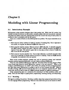
Fig. 1. Validation of engine torque model (18) on testing dataset. (Solid line: system output; dotted line: predicted output from the model.)
(18) (19) (20) (21) (22) are defined as
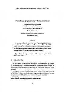
Fig. 2. Validation of HC model (19) on testing dataset. (Solid line: system output; dotted line: predicted output from the model.)
respectively. It should be noted that, as for most of the data-driven modeling work, the process of selecting the input variables for the model involved both applying physical LP-SVM-ARMA intuition and trial-and-error. In the case of engine modeling, we have applied our previous modeling experience in selecting input variables, and leveraged the flexibility of the linear programming problem formulation to define the model structure. for engine modBefore applying the LP-SVM-ARMA eling, several important parameters in the linear optimization problem (13), such as and , need to be selected. The kernel functions and adopted here for constructing the composite kernel are in the form of the GRBF kernel (5), and the values
of parameters and used for identifying the engine system models are listed in Table I. consists of multiple difConsider that the MA regressor ferent inputs to the system, and the values of one input may be orders of magnitude larger than that of another. Hence, it is usually necessary to use the technique of data standardization for scaling the input data with different distributions before the training process [30]. Through the training implemented by solving a linear programming problem, the engine models (18)–(22) can be obtained and further the models generated can be evaluated by validating on the testing dataset. The validation results are depicted in Figs. 1–5.
LU et al.: LINEAR PROGRAMMING SVM-ARMA
WITH APPLICATION IN ENGINE SYSTEM IDENTIFICATION
Fig. 3. Validation of NOX model (20) on testing dataset. (Solid line: system output; dotted line: predicted output from the model.)
851
Fig. 5. Validation of COV model (22) on testing dataset. (Solid line: system output; dotted line: predicted output from the model.)
TABLE II SPARSITY AND GENERALIZATION OF MODELS (18)–(22) LEARNED BY LINEAR PROGRAMMING SVM-ARMA
Fig. 4. Validation of catalyst temperature model (21) on testing dataset. (Solid line: system output; dotted line: predicted output from the model.)
The generalization performance of models can be evaluated by calculating the validation accuracy on the testing dataset measured by absolute root mean square error (RMSE)
linear programming SVM-ARMA model has excellent control of model complexity. In conjunction with the model sparsity, the validation accuracies of model (18)–(22) on the testing dataset are listed in Table II. For the sake of comparison, we also identify the dynamical engine system via the support vector regression with single kernel function [6], [31], in which the regressor is employed and the expansion on single kernel function
(23) (25)
and relative RMSE is used to represent the following five subsystems: (24) respectively, where is the output predicted by the obtained model and is the number of data in the testing dataset. RMSE is used as the key measure of model quality in this work, as the similar measure has been used for the engine modeling and powertrain control calibration community. The model sparsity shown in Table II, measured by the ratio of the number of support vectors to the number of training data points, indicates that
(26) (27) (28) (29) (30)
852
IEEE TRANSACTIONS ON AUTOMATION SCIENCE AND ENGINEERING, VOL. 8, NO. 4, OCTOBER 2011
TABLE III SPARSITY AND GENERALIZATION OF MODELS (26)–(30) LEARNED BY LP-SVR WITH SINGLE KERNEL
TABLE IV SPARSITY AND GENERALIZATION OF MODELS (26)–(30) LEARNED BY QP-SVR WITH SINGLE KERNEL Fig. 6. Validation of engine torque model (26) from LP-SVR on testing dataset. (Solid line: system output; dotted line: predicted output from the model.)
where
Fig. 7. Validation of HC model (27) from LP-SVR on testing dataset. (Solid line: system output; dotted line: predicted output from the model.)
In our simulation, the subsystems (26)–(30) are learned by LP-SVR and QP-SVR, respectively. The efficacy and generalization performance of the obtained kernel expansion model are evaluated by the model sparsity and validation accuracy on the testing dataset, which are listed in Table III and Table IV. Although the model sparsity listed in Table III is comparable to those in Table II, it is apparent that the modeling accuracies on testing datasets, which measure the generalization performance of models, are improved dramatically by using the LP-SVMARMA . Figs. 6–10 visualize the approximating performance of the models (26)–(30) built by LP-SVR on the testing dataset. The validation accuracies listed in Table IV commensurate with those in Table III; however, the sparsity of the models learned by QP-SVR degenerates severely, which leads to the forfeiture of model succinctness and thereby the inefficiency in evaluating the model outputs. In particular, the computationally burdensome requirement by quadratic programming makes it unpractical to model such a large size dataset generated by engine system via QP-SVR.
Fig. 8. Validation of NOX model (28) from LP-SVR on testing dataset. (Solid line: system output; dotted line: predicted output from the model.)
For evaluating the bias of each model learned by LP-SVM-ARMA , LP-SVR, and QP-SVR, the mean error on testing dataset for each model is also calculated and listed in the Table V.
LU et al.: LINEAR PROGRAMMING SVM-ARMA
WITH APPLICATION IN ENGINE SYSTEM IDENTIFICATION
Fig. 9. Validation of catalyst temperature model (29) from LP-SVR on testing dataset. (Solid line: system output; dotted line: predicted output from the model.)
Fig. 10. Validation of COV model (30) from LP-SVR on testing dataset. (Solid line: system output; dotted line: predicted output from the model.)
TABLE V MEAN ERRORS ON TESTING DATASET FOR MODELS LEARNED BY LP-SVM-ARMA , LP-SVR, AND QP-SVR
By comparing the data listed on the same row in Table V, it is apparent that the biases of models (18)–(22) learned by LP-SVM-ARMA are much less than the models (26)–(30) obtained by LP-SVR and QP-SVR, respectively. V. CONCLUSION The nature of LP-SVR is to use the kernel expansion as an ansatz for the solution, but to use a different regularizer, namely,
853
norm of the coefficients vector. In the comparison to the QP-SVR, it is evident that LP-SVR is superior in securing the succinctness of the model representation, which is of paramount importance in the practice of non-parametric systems identification. It is also noteworthy that the idea of norm minimization has recently attracted intensive interest in the emerging field of compressive sensing [32], [33]. Featured by the more flexible regressor structure, SVM-ARMA is capable of sculpting the different ways that AR and MA contribute to the output of the identified dynamical system by using the composite kernel. From the perspective of non-parametric statistical modeling, SVM-ARMA provides us a new avenue beyond the use of regularization term to control the model capacity through diminishing the predefined set of admissible functions. This is particularly useful in processing the input data with different properties, such as hyperspectral image [25]. On the other hand, the properties of the models obtained via SVM-ARMA are germane to the regularization term adopted and the corresponding optimization techniques employed. For the purpose of controlling the complexity of the model and improving the model sparsity, the norm of the coefficients vector in the kernel expansion is used as the regularization term in the proposed LP-SVM-ARMA approach, resulting in a linear optimization problem. Due to the superiority of linear programming technique over quadratic programming in terms of computational efficiency, LP-SVM-ARMA is more apt to be applied for modeling complex nonlinear dynamical systems. The advantages and potential of the developed LP-SVM-ARMA have been demonstrated in modeling an inline four cylinder engine system. The LP-SVM-ARMA model in its current format, also referred to as series-parallel format [34], is more suitable for prediction when the variables of interest are measurable. Its utility can be further expanded if the model can be implemented in the parallel format [35], where the delayed model output is used in the autoregression term. The efficacy of the parallel LP-SVM-ARMA model is currently under investigation, and will be a subject of the future publication. REFERENCES [1] T. Hofmann, B. Schölkopf, and A. J. Smola, “Kernel methods in machine learning,” Ann. Statistics, vol. 36, no. 3, pp. 1171–1220, 2008. [2] B. Schölkopf and A. J. Smola, Learning With Kernels: Support Vector Machines, Regularization, Optimization, and Beyond. Cambridge, MA: MIT Press, 2002. [3] V. Kecman, Learning and Soft Computing: Support Vector Machines, Neural Networks, and Fuzzy Logic Models. Cambridge, MA: MIT Press, 2001. [4] N. Cristianini and J. Shawe-Taylor, An Introduction to Support Vector Machines and Other Kernel-Based Learning Methods. Cambridge, MA: Cambridge Univ. Press, 2000. [5] A. J. Smola and B. Schölkopf, “A tutorial on support vector regression,” Statistics and Comput., vol. 14, pp. 199–222, 2004. [6] H. R. Zhang, X. D. Wang, C. J. Zhang, and X. S. Cai, “Robust identification of non-linear dynamic using support vector machine,” IEE Proc. Sci., Meas. Technol., vol. 153, no. 3, pp. 125–129, 2006. [7] W. C. Chan, C. W. Chan, K. C. Cheung, and C. J. Harris, “On the modeling of nonlinear dynamic systems using support vector neural networks,” Eng. Appl. Artif. Intell., vol. 14, pp. 105–113, 2001. [8] A. Gretton, A. Doucet, R. Herbrich, P. J. W. Rayner, and B. Schölkopf, “Support vector regression for black-box system identification,” in Proc. 11th IEEE Workshop on Statistical Signal Process., 2001, pp. 341–344.
854
IEEE TRANSACTIONS ON AUTOMATION SCIENCE AND ENGINEERING, VOL. 8, NO. 4, OCTOBER 2011
[9] B. R. Pramod and S. C. Bose, “System identification using ARMA modeling and neural networks,” J. Eng. Ind., vol. 115, pp. 487–491, 1993. [10] R. J. P. de Figueiredo and G. Chen, Nonlinear Feedback Control Systems: An Operator Theory Approach. New York: Academic Press, 1993. [11] Y. P. Zhao and J. G. Sun, “Multikernel semiparametric linear programming support vector regression,” Expert Systems With Applications, vol. 38, pp. 1611–1618, 2011. [12] O. L. Mangasarian and D. R. Musicant, “Large scale kernel regression via linear programming,” Mach. Learning, vol. 46, pp. 255–269, 2002. [13] J. P. Pedroso and N. Murata, “Support vector machines with different norms: Motivation, formulations and results,” Pattern Recognit. Lett., vol. 22, pp. 1263–1272, 2001. [14] J. Zhu, S. Rosset, T. Hasite, and R. Tibshirani, “1-norm support vector machines,” Neural Inform. Process. Syst., vol. 16, 2003. [15] O. L. Mangasarian, “Support vector machine classification via parameterless robust linear programming,” Optimization Methods and Software, vol. 20, pp. 115–125, 2005. [16] Z. Lu and J. Sun, “Non-Mercer hybrid kernel for linear programming support vector regression in nonlinear systems identification,” Appl. Soft Comput., vol. 9, no. 1, pp. 94–99, 2009. [17] Z. Lu, J. Sun, and K. Butts, “Linear programming support vector regression with wavelet kernel: A new approach to nonlinear dynamical systems identification,” Math. Comput. Simulation, vol. 79, no. 7, pp. 2051–2063, 2009. [18] S. H. Lee, R. J. Howlett, S. D. Walters, and C. Crua, “Modeling and control of internal combustion engines using intelligent techniques,” Cybern. Syst., vol. 38, pp. 509–533, 2007. [19] G. Bloch, F. Lauer, C. Guillaume, and C. Yann, “Support vector regression from simulation data and few experimental samples,” Inform. Sci., vol. 178, pp. 3813–3827, 2008. [20] T. Holliday, A. J. Lawrance, and T. P. Davis, “Engine-mapping experiments: A two-stage regression approach,” Technometrics, vol. 40, no. 2, pp. 120–126, 2009. [21] M. Martinez-Ramon, J. L. Rojo-Álvarez, G. Camps-Valls, J. Muñoz-Marí, A. Artes-Rodriguez, and A. R. Figueiras-Vidal, “Support vector machines for nonlinear kernel ARMA system identification,” IEEE Trans. Neural Networks, vol. 17, no. 6, pp. 1617–1622, Nov. 2006. [22] H. Wang, F. Sun, Y. Cai, and Z. Zhao, “Online chaotic time series prediction using unbiased composite kernel machine via Cholesky factorization,” Soft Comput., vol. 14, pp. 931–944, 2010. [23] M. Espinoze, J. A. K. Suykens, and B. De Moor, “Kernel based partially linear models and nonlinear identification,” IEEE Trans. Automatic Control, vol. 50, no. 10, pp. 1602–1606, Oct. 2005. [24] Z. Lu, J. Sun, and K. Butts, “Application of linear programming SVM ARMA for dynamic engine modeling,” in Proc. Amer. Control Conf., Baltimore, MD, 2010, Jun. 30–Jul. 2. [25] G. Camps-Valls, L. Gomez-Chova, J. Muñoz-Marí, J. Vila-Francés, and J. Calpe-Maravilla, “Composite kernel for hyperspectral image classification,” IEEE Geosci. Remote Sensing Lett., vol. 3, no. 1, pp. 93–97, Jan. 2006. [26] A. Nakashima and H. Ogawa, “How to design a regularization term for improving generalization,” in Proc. 6th Int. Conf. Neural Inform. Process., Perth, Australia, Nov. 1999, pp. 222–227. [27] A. Smola, B. Schölkopf, and G. Rätsch, “Linear programs for automatic accuracy control in regression,” in Proc. 9th Int. Conf. Artif. Neural Networks, Berlin, Germany, 1999, pp. 575–580. [28] B. Epstein, Orthogonal Families of Analytic Functions. New York: Macmillan, 1965. [29] J. A. Cook, J. Sun, J. H. Buckland, I. V. Kolmanovsky, H. Peng, and J. W. Grizzle, “Automotive powertrain control—A survey,” Asian J. Control, vol. 8, pp. 237–260, 2006. [30] S. Ghahramani, Fundamentals of Probability With Stochastic Processes, 3rd ed. Englewood Cliffs, NJ: Prentice-Hall, 2005. [31] Z. Lu and J. Sun, “Soft-constrained linear programming support vector regression for nonlinear black-box systems identification,” in Artificial Intelligence for Advanced Problem Solving Techniques, D. Vrakas and I. Vlahavas, Eds. Hershey, PA: Information Science Reference Publishing, Feb. 2008.
0
[32] R. G. Baraniuk, “Compressive sensing,” IEEE Signal Process. Mag., vol. 24, no. 4, pp. 118–121, Jul. 2007. [33] D. L. Donoho, “Compressed sensing,” IEEE Trans. Inform. Theory, vol. 52, no. 4, pp. 1289–1306, Apr. 2006. [34] P. Gupta and N. K. Sinha, “Neural networks for identification of nonlinear systems: An overview,” in Soft Computing and Intelligent Systems: Theory and Applications, N. K. Sinha and M. M. Gupta, Eds. New York: Academic Press, 1999. [35] O. Nelles, Nonlinear System Identification. Berlin, Germany: Springer-Verlag, 2000.
Zhao Lu received the M.S. degree in control theory and engineering from Nankai University, Tianjin, China, in 2000, and the Ph.D. degree in electrical engineering from the University of Houston, Houston, TX, in 2004. From 2004 to 2006, he worked as a Postdoctoral Research Fellow in the Department of Electrical and Computer Engineering, Wayne State University, Detroit, MI, and the Department of Naval Architecture and Marine Engineering, University of Michigan, Ann Arbor, respectively. Since 2007, he has been with the faculty of the Department of Electrical Engineering, Tuskegee University, Tuskegee, AL. His research interests mainly include machine learning, pattern recognition, and nonlinear control theory.
Jing Sun (M’89-SM’00-F’04) received the B.S. and M.S. degrees from the University of Science and Technology of China, Hefei, in 1982 and 1984, respectively, and the Ph.D. degree from the University of Southern California, Los Angeles, in 1989. From 1989 to 1993, she was an Assistant Professor with the Department of Electrical and Computer Engineering, Wayne State University. She joined the Ford Research Laboratory in 1993, where she worked in the Powertrain Control Systems Department. After spending almost ten years in industry, she returned to academia and joined the faculty of the College of Engineering, University of Michigan, in 2003, where she is now a Professor in the Department of Naval Architecture and Marine Engineering and the Department of Electrical Engineering and Computer Science. Her research interests include system and control theory and its applications to marine and automotive propulsion systems. She holds over 30 U.S. patents and has coauthored a textbook on Robust Adaptive Control. Dr. Sun is a recipient of the 2003 IEEE Control System Technology Award.
Kenneth Butts received the B.E. degree in electrical engineering from the General Motors Institute (now Kettering University), Flint, MI, the M.S. degree in electrical engineering from the University of Illinois, Chicago, and the Ph.D. degree in electrical engineering systems from the University of Michigan, Ann Arbor. He is an Executive Engineer in the Powertrain, Chassis, and Regulatory Division, Toyota Motor Engineering and Manufacturing North America, Ann Arbor, MI. In this position, he is investigating methods to improve engine control development productivity. He has worked in the field of automotive electronics and control since 1982, almost exclusively in research and advanced development of powertrain controls.