An application of mixed-integer linear programming models on the ...

OR Spectrum (2002) 24: 449–465 c Springer-Verlag 2002


An application of mixed-integer linear programming models on the redesign of the supply network of Nutricia Dairy & Drinks Group in Hungary Francisca H.E. Wouda1 , Paul van Beek2 , Jack G. A. J. van der Vorst3 , and Heiko Tacke4 1 2 3 4

Friesland Dairy&Drinks Group, Rijksweg 66, 2880 Bornem, Belgium Wageningen University, Operations Research & Logistics Group, Hollandseweg 1, 6706 KN Wageningen, The Netherlands Wageningen University, Management Research Group, Hollandseweg 1, 6706 KN Wageningen, The Netherlands ISAGRI Agrarsoftware, Eickerhoeh 1, 58553 Halver, Germany

Abstract. Between 1995 and 1998 Nutricia acquired a number of dairy companies in Hungary. Each of these companies produced a wide variety of products for its regional market. Although alterations had been made to the production system in the last few years, production and transportation costs were still substantial. This paper presents a research study with regard to the optimisation of the supply network of Nutricia Hungary using a mixed-integer linear programming model. Focussing on consolidation and product specialisation of plants the objective was to find the optimal number of plants, their locations and the allocation of the product portfolio to these plants, when minimizing the sum of production and transportation costs. The model is in line with traditional location/allocation models, with a modification concerning inter-transportation of semi-finished products between plants. The production costs used in this model are based on a Green field situation, taking into account new and more advanced technologies available today. The model is used by the Nutricia Dairy and Drinks Group as a decision supporting tool. Key words: Mixed-integer linear programming – Location/allocation – Economy of scale – Production/distribution – Scenario analysis

Correspondence to: F. H. E. Wouda

450

F. H. E. Wouda et al.

1 Introduction The Nutricia Dairy & Drinks Group (NDDG) has grown continuously since the beginning of its activities in Hungary in 1995. Since then a number of dairy companies with multiple plants has been acquired, each plant producing a wide range of products supplying dairy products to a specific region. In order to improve the logistic system and to reduce the production costs, the number of plants and the product portfolio were rationalised (resulting in three main brands, namely Milli, P¨otty¨os and Ok´e) and the distribution system was reconfigured. Nowadays, NDDG produces about 300 dairy products in different packages, different flavours and under different brand names; these are products like yoghurt, cheese, milk powder, fresh and long shelf-life milk, cream, butter and desserts. Although changes have been made to the system in the last few years, total system costs in Hungary are still too high due to a number of inefficiencies. NDDG wanted to evaluate a number of redesign strategies: • Regionalisation: each plant serves the customer with a full range of products within the region. • Consolidation: production is centralized at one plant and serves the whole country. • Product specialisation: each plant is producing a certain product group and serves the whole country (via several distribution centers). • Process specialisation: each plant is specialised in a certain stage of manufacturing, e.g. a plant for milk reception, for preparation and one for packing the product. The customers are served from the packaging plant. The objective of this research was to evaluate these strategies by identifying the optimal number of plants, their locations and the allocation of the product portfolio to these plants, when minimizing the sum of production and transportation costs. In literature, a number of models and procedures for the analysis of manufacturing strategies can be found (e.g. Cohen and Lee, 1989; Eppen et al., 1998; Krajewski and Ritzman, 1999). The contribution of this paper is first of all the modification that had to be made for the inter-transportation of semi-finished products between the plants. Secondly, it is an example of the applicability of Operations Research techniques in real life, since the model is actually used by a dairy company. The remaining part of this paper is structured as follows. First, in Section 2, the case analysis is described. In Section 3 the location/allocation model is formulated. Section 4 describes the results followed by the conclusions and discussion in Section 5.

2 Case analysis and demarcation Figure 1 presents an overview of the supply network considered in this research. Currently more than 400 farmers situated mostly in the eastern part of Hungary are supplying the 9 plants daily with raw milk. The size of the farms differ from 20 thousand liter to 11 million liter on annual basis, although there is a tendency that

An application of mixed-integer linear programming models

451

the small farms grow larger or disappear. Small farms deliver their milk to so called milk collecting points. The milk is collected by a transport company at these milk collecting points and directly at the larger farms. The 9 plants produce over 300 products. Some of the plants are already dedicated factories for a certain product group. During production semi-finished products are prepared. These semi-finished products (e.g. cream, whey, buttermilk, permeate) are transported to one of the other plants and processed into finished products. Since most of the products produced are fresh products, the production volume is strongly related to the daily demand of products. For some products like cheese, milk powder and long shelf-life milk an amount of stock is generated. Depending on the demand of certain products the daily inter-transport volumes vary. The products are forwarded to 17 distribution centres which are serving over 17.000 shops spread all over the country. In almost each county a distribution center is located, taking care of regional distribution to the shops. For some of the big retailer chains transport is done directly from the plant to the central distribution center of this retailer. A part of the production (e.g. cheese, milk powder in bulk and long shelf-life milk) is meant for export and for industrial customers. If we focus on this part of the supply network, the following cost factors can be identified: • Milk collection costs: raw milk is collected from the farmers until the milk collection truck has reached its maximum capacity. • Transportation costs of raw milk: after milk collection the milk is pumped into a bigger truck which will deliver the milk to the plant where it is needed. • Production costs: the raw milk is processed into finished products and semifinished products (like cream, whey, permeate and buttermilk). • Inter-transportation costs: the semi-finished products are transported in bulk to other plants where they are needed. • Transportation costs of finished products: the finished products are transported to the distribution centers or sometimes directly to the (industrial) customer. • Warehousing costs within the distribution centers are incurred for order picking and handling. All costs mentioned above will have impact on the number of plants to be opened, their location(s) and the allocation of products to these location(s). The number of locations is mainly influenced by the production costs; the more economy of scale within production, the lower the production costs per unit. According to Slack et al., (1998) there are two categories of stimuli influencing location decisions: supply-side influences and demand-side influences. In this case, the supply-side influences are mainly the transportation costs of raw milk and inter-transportation costs. The influences on the demand side are mainly transportation costs of finished products. Finally, the allocation of the product portfolio to plants is mainly determined by the trade-off between transportation costs and production costs. To model over 400 farmers, 300 products distributed via 17 distribution centers to more than 17.000 shops is very complex. Since this case study is used to find a long term strategy, a number of data aggregations have been made. The first aggregation of data is to consider the milk volumes, production volumes and sales

452

F. H. E. Wouda et al.

DC

customers

farmers Production

Transport finished products customers

Transport cream etc.

farmers

Transport raw milk

DC

Production

customers

farmers

customers

DC

Fig. 1. Supply network of a dairy company

volumes on a yearly basis. No day to day variations are taken into account. The raw milk volume is quite constant during the year. The milk is more concentrated in winter time, smaller volume but a higher protein and fat content than in summer time.

Aggregation of farmers into milk regions The farmers are grouped into geographical milk regions. The size of a milk region should not exceed a certain diameter or volume. The farmers are grouped according to this rule, resulting in 9 regions and per region a gravity point in milk volume is defined. Within the region the collection costs are calculated. The collection costs depend on the distance between the farms and the annual milk volume of the farms.

Aggregation of products The main criterion to put up the 300 products into a number of product groups was to combine products which can be produced using the same preparation and packaging equipment, resulting in 13 product groups (Walstra et al., 1998). Figure 2 depicts an overview of the production steps of dairy products. The first number of steps, from raw milk reception to standardisation, is the same for all product groups (see the dashed part of the process description in Fig. 2). The milk is standardised at the right fat content needed for production of a certain product. This can result in a surplus of cream or an additional need of cream if the fat content needed is higher than the current fat content of the raw milk. Additional cream is transported from another plant or surplus cream is transported to another plant. The first common part of the process is analysed separately from the other more specific processing and packaging steps. If a number of product groups is produced in one plant, economies of scale can be gained in the first common part of the process.

An application of mixed-integer linear programming models

Cream

Raw milk

Cooling

Thermisation & cooling

Separation

Homogeniser Standardisation

Skim milk

453

Other ingredients

Specific processing

Whey

Packaging materials

Specific packaging

Finished products

Permeate

Buttermilk

Fig. 2. Production chain of dairy products

Definition of production costs The costs per product group could be determined in the existing situation, but then it depends on the current capacity of the plant, the product portfolio, the efficiency achieved with the existing equipment etc. If the model determines the strategically optimal location(s) of plants and allocation of product groups, the product portfolio will most probably change. Also the capacity needed for a certain plant, will change. Besides that, it is the question if the existing equipment will be used in the long run. New and improved technologies should be considered. For this case study a method based on “Green field costs” is used. These are the costs associated with a Green field situation; define the capacity needed for a certain product group, invest in the newest and most advanced and proven equipment available today, arrange this into the most efficient layout of the plant and the needed utilities around it. Directly related to the choice of equipment is the need of direct personnel, the energy need and the maintenance cost of the equipment. For a number of capacities of plants the Green field investments and personnel level in 1, 2 and 3 shifts a day needed (direct and indirect) are determined together with the energy use and maintenance costs of the equipment. This result is presented in Figure 3 for one of the product groups. It turns out that the relation between total annual costs and annual capacity can be described very accurately by a fixed-charge linear cost function (Hax and Candea, 1984; Vidal and Goetschalckx, 2001). For each product group this linear cost function is determined and used in the model.

Aggregation of distribution centers & shops In the current situation, finished products are transported from all 9 plants to 17 distribution centers widely spread over Hungary. Most distribution centres serve their own region, but some are right next to the plant and serve their own region as well as other distribution centers and larger customers. Since on the long term the number and location of distribution centres is not stringent, the location and demand from customers (shops) is used. The shops are grouped into 20 geographical regions and per region a gravity point in sales volume is determined. These geographical

454

F. H. E. Wouda et al.

Total annual costs

y = 1238,4x + 1E+08 R2 = 0,985

Annual capacity

Fig. 3. Total annual costs of a Green field plant related to its annual capacity (the dots refer to the combination of capacity/shift options)

regions are the 19 counties of Hungary and Budapest. The gravity point is the capital of the county, since this is by far the biggest city in most of the counties.

3 MILP formulation of the location/allocation model The location-allocation problem could be described as: ‘What would be the optimal number, location and size of the production plants and what product groups should each plant produce, given the market demand and the milk supply, such that the total costs (comprising the production and transportation costs) are minimized.’ To solve this problem a location/allocation model is build consisting of an objective function and restrictions. The variables and the objective function of the model are described in Section 3.1. The restrictions are described in Section 3.2.

3.1 The variables and the objective function The variables used in the location/allocation model are defined below: Indices: i j,h k p

milk region (i = 1,2,...,I) location of plant (j,h = 1,2,...,J) sales region (k = 1,2,...,K) product group (p = 1,2,...,P)

An application of mixed-integer linear programming models

455

Variables: Xij PRODjp CREAMhj CRREQj CRSURPj SCREAMj WHEYhj WHREQj WHPRODj SWHEYj BUThj BUREQj BUPRODj SBUTj PERhj PEREQj PEPRODj SPERj Zjkp

amount of milk transported from region i to location j (in liters) amount of product p produced at location j (in pallets) amount of cream transported from location h to location j (in liters) net amount of cream required at location j (in liters) net amount of cream surplus at location j (in liters) surplus of cream in location j after transportation to lack locations (in liters) amount of whey transported from location h to location j (in liters) net amount of whey required at location j (in liters) net amount of whey produced at location j (in liters) surplus of whey in location j after transportation to lack locations (in liters) amount of buttermilk transported from location h to location j (in liters) net amount of buttermilk required at location j (in liters) net amount of buttermilk produced at location j (in liters) surplus of buttermilk in location j after transportation to lack locations (in liters) amount of permeate transported from location h to location j (in liters) net amount of permeate required at location j (in liters) net amount of permeate produced at location j (in liters) surplus of permeate in location j after transportation to lack locations (in liters) amount of product p transported from location j to depot k (in pallets)

Binary variables: YPRODjp YMILKj

binary decision variable for setting up a production line p at location j binary decision variable for setting up a milk reception at location j

Coefficients: mcci tcmij smrc mrc spcp pcp tcihj tcfjk mavi dkp ap skm crm crp kwhp bup pep bigpos

milk collection costs in region i (HUF per liter) milk transportation costs from region i to location j (HUF per liter) set-up costs milk reception (HUF) variable costs milk reception (HUF per liter) set-up costs production line product p (HUF) variable costs production of product p (HUF per pallet) transportation costs of semi-finished products from location h to j (HUF per liter) transportation costs finished products from location j to depot k (HUF per pallet) amount of milk available in region i (liters) demand of product p in sales region k (pallets) amount of skim milk required per pallet of product p (liters) skim milk percentage of the raw milk cream percentage of the raw milk amount of cream required per pallet of product p (liters) amount of whey required or produced per pallet of product p (liters) amount of buttermilk required or produced per pallet of product p (liters) amount of permeate required or produced per pallet of product p (liters) big positive number

456

F. H. E. Wouda et al.

X ij

i

PROD jp YPROD jp YMILK j

WHEYhj

i

CREAM hj

X ij

Z jkp

k

PROD jp YPROD jp PERhj

Z jkp

k

BUT hj

PROD jp YPROD jp

i X ij

YMILK j

PROD jp YPROD jp

k Z jkp

Fig. 4. Supply network with material flows and associated decision variables mxloc

maximum number of locations that should be opened

HUF (Hungarian Forint) is the currency of Hungary. 250 Hungarian Forints equal 1 Euro. The objective function can be described as follows: Minimize

{milk collection costs + milk transportation costs from region to plant + milk reception costs + production costs + transportation costs of inter-deliveries from plant to plant + transportation costs of finished products from plant to sales region}

In Figure 4 the network of the model is visualized. The model starts at the milk region i. In this region there are costs incurred to collect the milk and transport it to the gravity point of the milk region. The milk collection costs per liter differ per region i and are indicated by mcci . After collecting the milk, it is transported from the gravity point of region i to the plant. The transported volume from region i to location j is called Xij . The transportation costs of raw milk are defined as tcmij . If the binary variable Y M ILKj is equal to 1, there is a milk reception unit at location j. This results in set-up costs smrc and variable costs mrc. If the binary variable Y P RODjp is equal to 1, there is a production line of product p at location j. This results in set-up costs spcp and variable costs pcp for product p. The production volume of product p at location j is called P RODjp . For the production of product p, a certain amount of cream, whey, permeate or buttermilk could be required in addition to raw milk or a certain amount of them could be produced during production of product p. The amount required per location is called CRREQj , W HREQj , P EREQj or BU REQj respectively. When less cream, whey, permeate or buttermilk is required than produced at a location, there is a surplus called CRSU RPj , W HP RODj , P EP RODj and BU P RODj respectively. The lack of cream, whey, permeate and buttermilk is fulfilled by transporting the required amount from a surplus location. The intertransportation costs of these ‘semi-finished products’ from location h to location j

An application of mixed-integer linear programming models

457

are called tcihj . The amount of semi-finished products transported is indicated by CREAMhj , W HEYhj , BU Thj and P ERhj . In this case study the net amount of cream, whey, permeate and buttermilk in total is a surplus. It is left at the location where it is produced. The surpluses are indicated by SCREAMj , SW HEYj , SBU Tj and SP ERj respectively. In reality the surpluses will be converted into powder or butter in case of cream and are stored or sold to other companies, or the semi-finished products are sold as cattle feed. In the model no cost effects of these surpluses are taken into account, since they are negligible. Finally finished products p are transported to sales regions k, resulting in transportation costs tcfjk and material flows Zjkp . The model contains 126 binary variables, 2862 continuous variables and another 108 variables, which do not play a role in the objective function but in the restrictions. The optimisation has been carried out with the Xpress – MP optimisation system from Dash Optimization Ltd. Computing times varied from 15–60 minutes depending on the scenario (for scenarios see Table 1). In mathematical form the objective function can be written as:       smrc · Y M ILKj + (mcci + mrc + tcmij ) · Xij       j i j         + spc · Y P ROD   p jp     p j       + pc · P ROD p jp (1) min p    j       + tcihj · (CREAMhj + W HEYhj + P ERhj + BU Thj )        h j            tcfjk · Zjkp +  j

p

k

3.2 Restrictions The model should take into account certain restrictions. For example, demand should be satisfied by production and milk supply from a region must not exceed the amount of milk available in that region. There are restrictions for milk transport, milk reception, production, inter-transport, transportation of finished products and possible plant locations. The restrictions are explained below. Milk transportation and milk reception The transported amount of milk from region i to location j cannot exceed the amount of milk available in region i: Xij ≤ mavi , for all i (2) j

Location j can only process raw milk if it has a milk reception unit: Xij ≤ bigpos · Y M ILKj , for all j i

(3)

458

F. H. E. Wouda et al.

Production The supplied amount of milk must equal the amount of milk required for production at location j: skm · Xij = ap · P RODjp , for all j (4) p

i

Location j can only produce product group p if it has a production line for p: P RODjp ≤ bigpos · Y P RODjp ,

for all j, p

(5)

The amount of net cream required or surplus at location j is defined by the following formula: CRREQj −CRSU RPj = crp · P RODjp − crm · Xij , for all j (6) p

i

The amount of net whey required or produced at location j is defined by the following formula: W HREQj − W HP RODj = whp · P RODjp , for all j (7) p

The amount of net buttermilk required or produced at location j is defined by the following formula: BU REQj − BU P RODj = bup · P RODjp , for all j (8) p

The amount of net permeate required or produced at location j is defined by the following formula: P EREQj − P EP RODj = pep · P RODjp , for all j (9) p

Since all variables must be positive or zero, each location j has a requirement for semi-finished products or a surplus.

Inter-transport The transported amount of cream from j to h should not exceed the surplus: CREAMjh ≤ CRSU RPj , for all j (10) h

The transported amount of cream from h to j must satisfy the requirement of cream at location j: CREAMhj = CRREQj , for all j (11) h

An application of mixed-integer linear programming models

459

The net surplus of cream at location j after transportation to location h is defined by the following formula: CREAMjh , for all j (12) SCREAMj = CRSU RPj − h

The transported amount of whey from j to h must not exceed the surplus: W HEYjh ≤ W HP RODj , for all j

(13)

h

The transported amount of whey from h to j must satisfy the requirement of whey in location j: W HEYhj = W HREQj , for all j (14) h

The net surplus of whey at location j after transportation to location h is defined by the following formula: W HEYjh , for all j (15) SW HEYj = W HP RODj − h

The transported amount of buttermilk from j to h must not exceed the surplus: BU Tjh ≤ BU P RODj , for all j (16) h

The transported amount of buttermilk from h to j must satisfy the requirement of buttermilk in location j: BU Thj = BU REQj , for all j (17) h

The net surplus of buttermilk at location j after transportation to location h is defined by the following formula: BU Tjh , for all j (18) SBU Tj = BU P RODj − h

The transported amount of permeate from j to h must not exceed the surplus: P ERjh ≤ P EP RODj , for all j (19) h

The transported amount of permeate from h to j must satisfy the requirement of permeate in location j: P ERhj = P EREQj , for all j (20) h

The net surplus of permeate at location j after transportation to location h is defined by the following formula: P ERjh , for all j (21) SP ERj = P EP RODj − h

460

F. H. E. Wouda et al.

Transportation of finished products The total amount of finished products transported to all gravity points k must equal the production: Zjkp = P RODjp , for all j, p (22) k

The production of product p must be equal to the demand of product p (with dkp the demand of product p in gravity point k): Zjkp = dkp , for all k, p (23) j

Restricted number of possible plant locations The maximum number of locations (mxloc) can be established by the following formula: Y M ILKj ≤ mxloc (24) j

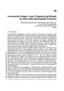
4 Scenarios and results The model is used to evaluate a number of different scenarios: • Scenario 0: current situation using Green field production costs. • Scenario 1: running the model without any additional restrictions to calculate the optimal solution using the current 9 locations. • Scenario 2: running the model with 4 other potential locations. In the long term, concerning Green field production sites, the dairy company is not bounded to use its existing locations only. If a new plant is build this could take place at another location. • Scenario 3: running the model with one of the optimal locations left out of the possible locations. One of the locations chosen at the optimal solution is taken out of the possible locations to show the second best option and its cost effects. • Scenario 4: running the model with production of a certain product group forced at a specific location. • Scenario 5: running the model with a fixed number of possible plants, namely 1 or 2. With restriction (24) the model is forced to open not more than a certain number of locations. In this case the effect is calculated if mxloc = 1 and if mxloc = 2. • Scenario 6: running the model closing one plant in the current situation. This way, the cost effects of closing a certain plant in the current situation are calculated. Because of the confidentiality of this research, the results cannot be discussed in detail. The results are summarised in Table 1. In Figure 5 an overview of the costs per scenario is presented.

An application of mixed-integer linear programming models

461

Table 1. Model results of scenario evaluations Scenario

Number of plants and location

Product portfolio

0 1

locations A, B, C, D, E, F, G, H and I locations A, B and C

2

locations A, B and C

3

locations A, B and D

4

locations A, B, C and E

5, mxloc = 1

location C

5, mxloc = 2

locations A and C

6

locations A, B, D, E, F, G, H and I

Each product group is produced at one or more locations. Each product group is produced at one location. Each product group is produced at one location. Each product group is produced at one location. Each product group is produced at one location. Each product group is produced at one location. Each product group is produced at one location. Each product group is produced at one or more locations.

Result scenario 0 and 6: The model only determines the flow of raw milk, semi-finished products and finished products. The costs are calculated with the nine current locations and for the situation that location C is closed. Result scenario 1: The optimal solution in this case-study is three locations. The product groups are allocated in such way that each product group is produced only at one location. A certain level of consolidation and product specialisation is taking place. The locations are specialized in a number of product groups. The product groups requiring a large amount of milk are located near to the largest volume in milk. Product groups requiring less milk are located closer to the market. There is still a certain volume of inter-transport, but less than in the current situation. Result scenario 2: The model does not choose to open one of the alternative locations. The results are the same as in scenario 1. The alternative locations considered are not better locations than the already existing locations. Result scenario 3: If one of the locations chosen by the model in the optimal solution is taken out of the possible locations (location C), the model determines the second best option. The model still opens three locations, A, B and D. Some product groups of the location taken out are deployed at one of the two other optimal locations. The other product groups are deployed at the new location. Result scenario 4: If a certain product group is forced at a certain location, E, the model decides to

462

F. H. E. Wouda et al.

Total costs

Milk collection Transport raw milk Intra transport Transport finished products Milk reception Production

9 locations

8 locations

4 locations

3 locations

3 locations

2 locations

1 location

Scenario 0

Scenario 6

Scenario 4

Scenario 1

Scenario 3

Scenario 5

Scenario 5

Scenario and number of locations opened

Fig. 5. Production and transportation costs per scenario

open 4 locations, A, B, C and E. The product group forced is the only product group produced at this fourth location. The other product groups are produced at the same location as in the optimal solution.

Result scenario 5: In this scenario the model is forced to open one location and a second time to open two locations. In case of two locations, the model chooses two of the locations of the optimal solution, A and C. The product groups of the third (closed) location (B) are deployed at the nearest location C. In case of one location, all product groups are allocated also at one of the optimal locations, the one in between the largest milk volume and the largest market, location C. Reducing the current number of production locations to a lower number of production locations decreases total costs. This applies especially to the production costs due to more product specialisation. If a product group is produced only at one location, the maximum attainable economy of scale is reached. Additional synergy can be reached by more economy of scale in milk reception. The milk reception costs are reduced if the number of locations is reduced, since every location has its own milk reception unit. The larger this milk reception unit, the more economy of scale can be gained. If less than three locations are opened, the milk reception costs decrease but the transportation costs increase. Especially the transportation costs for raw milk. The transportation costs of finished products slightly increase. The inter-transportation costs decrease, but their contribution to the total costs is not substantial. The milk collection costs are approximately the same in every scenario since almost all the milk is used for production.

An application of mixed-integer linear programming models

463

Sensitivity analysis Assumptions are made to calculate the transportation and the production costs. Does the result of the model change when these costs are higher or lower than calculated? A sensitivity analysis is carried out to check the consequences of these assumptions. 1. Production and milk reception costs: production is responsible for the major part of total cost. A 10% change in production costs has no impact on the outcome of the model. If the milk reception costs are increased by 30%, only two locations are opened instead of three. The same solution as in scenario 5 with locations A and C is optimal in this case. If the milk reception costs are reduced by 30%, a fourth location is opened (A, B, C and D) and certain product groups are deployed at this fourth location. A change of 10% in milk reception costs showed no effect. 2. Milk transportation costs. If the transportation costs of raw milk are increased by 5% again three locations are opened. However, one of the plant locations is changed as well as the allocation of product groups (locations A, B and D). If the transportation costs of raw milk are increased by 30% a fourth location is opened (locations A, B, C and D). A reduction in raw milk transportation costs showed no effect. 3. If the transportation costs of finished products are reduced by 10%, the same change takes place as in the increase of the transportation costs of raw milk by 5%. An increase up to 30% showed no effect. 4. A change in inter-transportation costs showed no effect. The model makes a trade-off between transportation costs and economies of scale in production and milk reception. The production costs decrease when product specialisation takes place. The milk reception costs decrease if the number of production locations is reduced. However, the total transportation costs increase when fewer locations are opened. At a certain point the additional transportation costs have reached the same level as the economies of scale advantage in the production costs. If fewer locations are opened for production, the total transportation costs increase more than the milk reception costs decrease, so the total costs increase. At the point of three locations opened, there is an optimum in total costs. This optimum is easily influenced by a small change in transportation costs. The number of opened locations calculated by the model is 2, 3 or 4 of the locations A, B, C and D. Locations E, F, G, H and I are not chosen by the model, only if the model is forced to. A more refined and detailed study towards transportation costs is necessary before the optimal number and location of production locations can be concluded more precisely. Also important are future expectations on milk supply and market demand, will there be a shift towards other regions of milk suppliers or demand, new product groups, rejection of product groups etc. In this study the current milk volume and sales numbers are taken as granted. If this changes it can certainly influence the optimal solution.

464

F. H. E. Wouda et al.

5 Conclusions This paper discusses a mixed integer linear programming model that was developed in cooperation with the Nutricia Dairy and Drinks Group. The model was used in a real life case to identify the optimal number of plants in Hungary, its locations and the allocation of the product portfolio to these plants, when minimizing the sum of production and transportation costs. The model showed its applicability in the decision making process, although a more refined and detailed study towards transportation costs is necessary as was suggested. The model determined which strategy to follow and at which location. Every investment proposal is compared to see if it fits into this strategy. Step by step a plan will be developed to come closer to the optimal solution. In case of new acquisitions by the NDDG the model can serve again to find the optimal solution including the new milk, product portfolio and market volume acquired together with new possible production locations. The same study could also be carried out for a wider area, e.g. which production strategy to follow in central Europe, western Europe or even whole Europe. In this case more cost factors should be taken into account, e.g. differences per country in milk prices, wages, taxes and in some cases custom duties. Since central European countries will join the EU in the future, the custom duties will disappear. The model itself can be further extended for future purposes. A first extension could be to decouple the specific preparation and specific packaging process steps in the Green field production costs. Some product groups are using the same preparation but other packaging equipment and other product groups are using other preparation but the same packaging equipment. By combining certain product groups in one factory, more economies of scale in production costs could be realized. Although, there is a certain limit to the economies of scale in production. When a production location produces more and more product groups the managerial complexity increases. This increase in complexity could cause an increase of production costs per unit of product. In the model this could be solved by adding a restriction to the number of product groups produced at one location. A second advantage of decoupling the preparation and packaging process steps is the possibility to switch towards a strategy of process specialisation instead of product specialisation. In the presented model the raw milk is directly linked to the production of product p by restriction (4). There is no inter-transportation of standardised milk built into the model to make process specialisation possible. The model should be adjusted for this and the split between preparation and packaging. This way the inter-transportation will play a more important role. This model is meant as and is used as a decision-supporting tool. It quantifies, evaluates, verifies and supports ideas and ‘gut feeling’. Of course, a lot of other quantifiable (e.g. social costs, disinvestments costs) as well as non-quantifiable factors (e.g. political, social, environmental, quality factors) play a role in decisionmaking. This model is meant to point out a direction, to get closer to the optimal situation and thus decrease total costs.

An application of mixed-integer linear programming models

465

References Cohen MA, Lee HL (1989) Resource deployment analysis of global manufacturing and distribution networks. Journal of Manufacturing and Operations Management 2: 81– 104 Eppen GD, Gould FJ, Schmidt CP Moore JH Weatherford LR (1998) Introductory management science, 5th edn. Prentice Hall, Upper Saddle River, NJ Hax AC, Candea D (1984) Production and inventory management. Prentice Hall, Upper Saddle River, NJ Krajewski LJ, Ritzman LP (1999) Operations management – strategy and analysis, 5th edn. Addison Wesley Longman, Reading, MA Slack N, Chambers S, Harland C, Harrison A, Johnston R (1998) Operations management, 2nd edn. Financial Times, Pitman, London Vidal CJ, Goetschalckx M (2001) A global supply chain model with transfer pricing and transportation cost allocation. European Journal of Operational Research 129: 134–158 Walstra P, Geurts TJ, Noomen A, Jellema A, Van Boekel MAJS (1998) Principles of dairy technology. Dekker, New York