until tunnel vision and finally blindness results. Patients diagnosed with the ... vision. In some cases the treatment is successful, resulting in the patient's vision.
An Application of Machine Learning Techniques for the Classification of Glaucomatous Progression Mihai Lazarescu, Andrew Turpin, and Svetha Venkatesh Department of Computer Science, Curtin University GPO Box U1987, Perth 6001, Australia {lazaresc,andrew,svetha}@computing.edu.au
Abstract. This paper presents an application of machine learning to the problem of classifying patients with glaucoma into one of two classes:stable and progressive glaucoma. The novelty of the work is the use of new features for the data analysis combined with machine learning techniques to classify the medical data. The paper describes the new features and the results of using decision trees to separate stable and progressive cases. Furthermore, we show the results of using an incremental learning algorithm for tracking stable and progressive cases over time. In both cases we used a dataset of progressive and stable glaucoma patients obtained from a glaucoma clinic.
1
Introduction
Machine learning techniques have been used successfully in a number of fields such as engineering [2] and multimedia [6]. Another important field where machine learning has been applied with considerable success is in medicine for tasks such as patient diagnosis [3]. Glaucoma is a disease that affects eye sight, and is the third most common cause of blindness in the developed world, effecting 4% of people over the age of 40 [10]. The vision loss associated with glaucoma begins in peripheral vision, and as the disease progresses vision is constricted until tunnel vision and finally blindness results. Patients diagnosed with the disease usually undergo treatment which may prevent further deterioration of their vision. In some cases the treatment is successful, resulting in the patient’s vision being stabilized. Unfortunately in some cases the treatment is not successful, and the visual field continues to constrict over time. One aim of the research in this field is to distinguish between stable glaucoma patients and progressive glaucoma patients as early in the life of the disease as possible. This allows ophthalmologists to determine if alternate treatments should be pursued in order to preserve as much of the patient’s sight as possible. With current techniques, vision measurements must be taken at regular intervals for four to five years before progression can be determined [5]. Most research on automatic diagnosis of glaucoma has concentrated on using statistical methods such as linear discrimination functions or Gaussian classiT. Caelli et al. (Eds.): SSPR&SPR 2002, LNCS 2396, pp. 243–251, 2002. c Springer-Verlag Berlin Heidelberg 2002 �
244
Mihai Lazarescu et al.
fiers [4, and references therein]. In this previous work, the data available combines information from several standard opthalmologic tests that assess both vision and damage to the optic nerve over time. Typical patient data has a series of observations collected at 6 monthly or yearly intervals, with each observation containing over 50 attributes. Because of the complexity of the data, many of the methods used for classification focus on the time series of a single attribute. [9] presents a comparison of several machine learning techniques such as linear support vector machines and point-wise linear-regression for data covering 8 sets of observations. [4] describes a study of 9 classification techniques but with data that covered only a single set of observations (no temporal data was available). A different approach that is based on the use of the optical disk features extracted from 3D eye scans is described in [1]. In this paper we present an approach that uses two types of learning: onestep learning that involves the use of decision trees; and incremental learning that uses a concept tracking algorithm. In both cases the processing involves a pre-processing step, where a number of new attributes are extracted from the data, and then application of one of the two learning approaches. We describe our method to extract the features from the data in detail below, and present the results obtained from applying the two learning methods to a medical dataset. The main contributions of this paper are the formulation of new features that enables the application of decision trees to separate out stable and progressive glaucoma, and the use of incremental learning to track changes in the two classes of patients. The paper is organized as follows. In Section 2 we describe the data used in the research. Section 3 presents the features extracted from the data. In Section 4 we present our results, and conclusions are presented in Section 5.
2
The Data
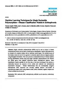
The data we used in our experiments consisted of the raw visual field measurements for glaucoma patients. A visual field measurement records the intensity of a white light that can be just seen by a patient in 76 different locations of the visual field. In order to collect the data, the patient is instructed to fixate on a central spot, and lights of varying intensities are flashed throughout the 76 locations in the visual field. The patient is instructed to push a button whenever they see a light. Figure 1(b) shows the output of the machine that was used to collect the data for this data set (Humphrey Field Analyzer I, Humphrey Systems, Dublin CA). A high number (30 or above) indicates good vision in that location of the field. A score of zero at a location indicates blindness at that location. If a patient’s glaucoma is progressing over time, therefore, we would expect a decrease in some of the numbers in their visual field measurement. For each patient, 6 visual field measurements are available each of which is made at an interval of 6 months. All measurements were adjusted prior to our processing to represent right eyes of 45 year old patients. The data was provided by Dr. Chris Johnson from Devers Eye Institute, Portland, Oregon.
An Application of Machine Learning Techniques
245
31 30 29 30
17 17 18 18 17 17 17 17 18 19 5
16 16 16 16 17 18 19 20
2
30 31 32 29 29
4
32 32 30 27 29 28
15 15 15 15 15 14 16 19 20 20
29 31 31 32 28 31 32 30 29 30
14 14 14 14 13 s12 13 0 8 8 8 8 9 10 10 0 7
1
1
28 27 29 30 29 s31 31 0 28 29 30 28 31 30 31 0
2
27 31 30 29 29 29 27 31 28 27
21 21
7
7
7
7
8
7
3
2
6
6
6
6
5
4
3
3
5
5
5
4
4
3
5
4
4
4
(a)
27 30 29 31
32 29 30 29 31 30 29 29 29 28 28 31 32 31 27 32 32 29 (b)
Fig. 1. (a) A map identifying the nerve fiber bundles for each visual field location. (b) A sample visual field measurement
We also made use of a map of the nerve fiber bundles as they are arranged in the retina [11], as shown in Figure 1(a). Each location of our visual field is numbered on the map according to which nerve fiber bundle it belongs. If glaucomatous damage occurs to one nerve fiber bundle, it is expected that all locations on that bundle will have decreased visual field thresholds. All the data had been previously labeled as either stable or progressive by experts. A fact worth noting is that the data is very noisy, as is widely reported in the opthalmologic literature [8, and references therein]. One obvious source of the noise is that human responders make mistakes: they press the button when they don’t see a light, they don’t press the button when they do see a light, or they do not fixate on the central spot. Another more insidious source of noise is that the patient’s criteria for pushing the button (that is, determining if they have “seen” the light or not) can change during a test, and between different tests. Hence the patients with the same condition will likely produce different responses. It is worth noting here that there are other types of data that could be used to classify patients. These include other measures of the visual field and structural measures of the retina and optic nerve. At present there is no universally accepted definition of glaucomatous progression, and various on-going clinical drug trials use their own set of criteria and definitions to determine outcomes. However, all current schemes for determining progression have one thing in common: they use visual field data such as the type described above.
3
The Features Extracted
Several approaches have been used in the past to classify visual field data. One such approach is to consider each individual visual field measurement for each observation as a separate attribute, thus creating a total of 456 attributes (76x6) [9].
246
Mihai Lazarescu et al.
A popular approach is to consider the data to have 76 attributes and then to use statistical methods such as linear regression to determine whether the visual field response decreases over time. Our initial attempts also used the latter approach but the results were disappointing when combined with decision trees. Therefore, we decided to derive a new set of features. Unlike previous approaches, that used trends in the individual visual field measurements, we attempted to derive a set of features that can be obtained with ease, and that can be easily understood by glaucoma researchers. To obtain meaningful features we made extensive use of common knowledge about glaucoma, including: – a consistent decrease in the response from a nerve fiber bundle indicates that the disease is progressing; – a large decrease in the overall response indicates that the disease is progressing – an increase in the anomalous readings of the eye over time indicates that disease is progressing; – a low response for nerve fiber bundle 0 does not indicate glaucoma as it is the blind spot for the eye; – nerve fiber bundles can be grouped to gain a better picture of progression; – the nerve fiber bundles closest to the nose are more likely to show early loss due to glaucoma; We extracted two types of features. Type 1 (seven features) uses information from only a single observation while type 2 (five features) describes the temporal aspects of the data. The features of type 1 are described below. – Feature 1–Overall eye response. Computed by obtaining the average of the 76 visual field measurements. – Feature 2–Existence of an anomaly–for each location in the visual field, compare its value to the median value in a 3x3 neighborhood. If the value is greater or equal with the median, then no anomaly is indicated and feature 2 is set to 0. If the value is smaller than the median, and the difference between the pixel and at least 6 of the neighbors is larger than a threshold, then an anomaly is deemed to exist and feature 2 is set to 1. The neighborhood is set to 2x2 at the border of the visual field. – Feature 3—Number of anomalies per optic nerve bundle. Each pixel in the visual field corresponds to one of the 21 nerve fiber bundles. Feature 2 is now amalgamated to get the number of anomalies per optic nerve. – Feature 4—Quadrant anomalies. The 10x10 region of the eye is divided into 4 quadrants (5x5 each) and Feature 2 is amalgamated for each quadrant.
An Application of Machine Learning Techniques
247
– Feature 5—Eye response per quadrant. Computed by averaging the visual field measurement values for each of the 4 quadrants. – Feature 6—Blind spot data. The value of the amalgamated score (from feature 3) for nerve fiber bundle 0 is indicative of the blind spot data. Feature 6 is set to this value. – Feature 7—Number of anomalies for 3 quadrants. The bottom right quadrant for this dataset was ignored because of the blind spot. The blind spot position varies from measurement to measurement because the data is noisy (patient’s may not sit in exactly the same spot for every test). Hence any anomaly discovered in this quadrant may in fact indicate the blind spot. Type 2 features were designed to capture the progression of the visual field responses over time. We specifically searched for consistency in the individual nerve fiber responses, the grouped nerve fiber responses, the overall change in the eye response and the number of anomalous visual responses in the eye. These include: – Feature 8—Average difference in eye response. Computed by taking the difference between the overall eye response at two time instances. – Feature 9—Change in anomalies per optic nerve bundle. This feature indicates whether or not a net difference has occurred for a nerve fiber bundle between two time instances. The time instances need not be consecutive. – Feature 10—Change in eye response for 3 quadrants. This feature indicates whether or not a net difference has occurred for the three quadrants (feature 7) between two time instances. – Feature 11—Difference in anomalies per optic nerve. This feature is computed by taking the difference between the number of anomalies for two consecutive times instances for the same optic nerve. – Feature 12—Difference in anomalies per quadrant. This is computed by taking the difference between the the anomalies for each quadrant for two consecutive time instances.
4 4.1
Results Classification Using Decision Trees
The instances containing the raw visual field measurements were processed to extract the 12 features and the data was split into 2 sets: a training and a test set. To classify and test the data we used the C4.5 (Release 8) software. The process was repeated 50 times and each time a different random training and test set was used. C4.5 generated decision trees that on average had 15 nodes
248
Mihai Lazarescu et al.
Table 1. Classification accuracy of the data using C4.5 and our 12 features CLASS STABLE PROGRESSIVE TOTAL FALSE POSITIVE 18 108 126 FALSE NEGATIVE 93 129 222 TRUE POSITIVE 299 432 731 RECALL % 95 83 89 PRECISION % 83 72 77
using 7 features consistently (all features were used but 5 of the features were not used with any consistency). The results are shown in Table 4.1. It can be seen that both the precision and recall for the stable class (95% and 82.5%) are higher than for the progressive class (83% and 72%). We examined the decision trees to determine the features that best defined the stable and the progressive cases. We found that features that were consistently used in all decision trees were: average difference in eye response (feature 8), change in eye response for 3 quadrants (feature 10), number of anomalies for 3 quadrants (feature 7), quadrant anomalies (feature 4) and difference in anomalies per quadrant (feature 12).
Fig. 2. Plot of the true-positive, false-positive and false-negative over the last four stages of the experiment for the stable class (each stage is equal to 10 time units)
An Application of Machine Learning Techniques
249
Fig. 3. Plot of the true-positive, false-positive and false-negative over the last four stages of the experiment for the progressive class (each stage is equal to 10 time units)
4.2
Using Incremental Learning to Track Patient Condition
We also investigated whether incremental learning could be used to classify a patient’s condition over time. To track the patient’s condition we used an incremental learning algorithm [7] that uses multiple windows to track the change in the data and adjust concept definitions. Because of the use of multiple windows, the system has the advantage that it can track changes more accurately. In data set for consisted of pairings of time instances: (1,2), (2,3), (3,4), (4,5) and (5,6). The pairings described the patient’s condition over a period of 3 years. The data is divided into 2 sets: a training set and a test set. Using the first pairing, the system builds the concepts for the progressive and stable class. These are concepts are progressively refined over four stages using subsequent samples from the training data. The system used the time pairing (2,3) for stage 1, (3,4) for stage 2, (4,5) for stage 3 and (5,6) for stage 4. The accuracy of the concepts is tested over the four stages using data from the test set. The resulting true-positive, false-positive and false-negative classification for the two classes in shown in Figures 3 and 2. The results obtained show that the system’s true-positive performance improved over time for the stable class. In the first two stages, the system classified the progressive and stable cases with 60% accuracy. In the last two stages the system averaged around 70% accuracy for the stable class. This was expected as the data covering the progressive patient is a lot more noisy than the stable cases. When comparing the performance of the incremental learning method to
250
Mihai Lazarescu et al.
the one-step learning using C4.5, the latter method is more accurate. However, the difference between the methods is not large which indicates that incremental learning could be used for the classification task especially as the method we used was based on simple k-means clustering.
5
Conclusion
In this paper we present an application of machine learning techniques to the problem of classifying patients that have either stable or progressive glaucoma. The work described in this paper involves both one-step and incremental learning. We extract 12 features based on knowledge gleaned from domain experts, and applied simple machine learning techniques (decision trees and incremental learning) to solve the problem of interpreting complex medical data. The approach described in this paper shows particular promise and that decision trees can be used to classify a patient’s condition as stable or progressive using some very simple features. The features are obtained from raw visual field measurements, and do not involve any significant processing to extract. The results indicate that by using features that do not concentrate on individual visual field measurements, a good classification performance can be obtained.
References 1. D. Broadway, M. Nicolela, and S. Drance. Optic disk appearances in primary open-angle glaucoma. Survey of Ophthalmology, Supplement 1:223–243, 1999. 244 2. P. Clark. Machine learning: Techniques and recent developments. In A. R. Mirzai, editor, Artificial Intelligence: Concepts and Applications in Engineering, pages 65– 93. Chapman and Hall, 1990. 243 3. R. Dybowski, P. Weller, R. Chang, and V. Gant. Prediction of outcome in critically ill patients using artificial neural networks synthesised by genetic algorithms. Lancet, 347:1146–1150, 1996. 243 4. M. Goldbaum, P. Sample, K. Chan et.al. Comparing machine learning classifiers for diagnosing glaucoma from standard automated perimetry. Investigative Ophthalmology and Visual Science, 43:162–169, 2002. 244 5. J. Katz, A. Sommer, D.E. Gaasterland, and D.R. Anderson. Analysis of visual field progression in glaucoma. Archives of Ophthomology, 109:1684–1689, 1991. 243 6. M. Lazarescu, S. Venkatesh, and G. West. Incremental learning with forgetting (i.l.f.). In Proceedings of ICML-99 Workshop on Machine Learning in Computer Vision, June 1999. 243 7. M. Lazarescu, S. Venkatesh, G. West, and H.H. Bui. Tracking concept drift robustly. In Proceedings of AI2001, pages 38–43, February 2001. 249 8. P.G.D. Spry, C.A. Johnson, A.M. McKendrick, and A. Turpin Determining progressiong in glaucoma using visual fields. In Proceedings of the 5th Asia-Pacific Conference on Knowledge Discovery and Data Mining (PAKDD2001, April 2001. 245 9. A. Turpin, E. Frank, M. Hall, I. Witten, and C.A. Johnson. Determining progressiong in glaucoma using visual fields. In Proceedings of the 5th Asia-Pacific Conference on Knowledge Discovery and Data Mining (PAKDD2001, April 2001. 244, 245
An Application of Machine Learning Techniques
251
10. J.J. Wang, P. Mitchell, and W. Smith. Is there an association between migraine headache and open-angle glaucoma? Findings from the Blue Mountains Eye Study. Ophthalmology, 104(10):1714-9, 1997. 243 11. J. Weber, and H. Ulrich. A perimetric nerve fibre bundle map. International Ophthalmology, 15:193–200, 1991. 245