An Application of Stochastic Programming in Solving Capacity

Hindawi Publishing Corporation Mathematical Problems in Engineering Volume 2015, Article ID 741329, 16 pages http://dx.doi.org/10.1155/2015/741329

Research Article An Application of Stochastic Programming in Solving Capacity Allocation and Migration Planning Problem under Uncertainty Yin-Yann Chen and Hsiao-Yao Fan Department of Industrial Management, National Formosa University, Yunlin 632, Taiwan Correspondence should be addressed to Yin-Yann Chen; [email protected] Received 31 August 2015; Revised 29 October 2015; Accepted 10 November 2015 Academic Editor: Yan-Jun Liu Copyright © 2015 Y.-Y. Chen and H.-Y. Fan. This is an open access article distributed under the Creative Commons Attribution License, which permits unrestricted use, distribution, and reproduction in any medium, provided the original work is properly cited. The semiconductor packaging and testing industry, which utilizes high-technology manufacturing processes and a variety of machines, belongs to an uncertain make-to-order (MTO) production environment. Order release particularly originates from customer demand; hence, demand fluctuation directly affects capacity planning. Thus, managing capacity allocation is a difficult endeavor. This study aims to determine the best capacity allocation with limited resources to maximize the net profit. Three bottleneck stations in the semiconductor packaging and testing process are mainly investigated, namely, die bond (DB), wire bond (WB), and molding (MD) stations. Deviating from previous studies that consider the deterministic programming model, customer demand in the current study is regarded as an uncertain parameter in formulating a two-stage scenario-based stochastic programming (SP) model. The SP model seeks to respond to sharp demand fluctuations. Even if future demand is uncertain, migration decision for machines and tools will still obtain better robust results for various demand scenarios. A hybrid approach is proposed to solve the SP model. Moreover, two assessment indicators, namely, the expected value of perfect information (EVPI) and the value of the stochastic solution (VSS), are adopted to compare the solving results of the deterministic planning model and stochastic programming model. Sensitivity analysis is performed to evaluate the effects of different parameters on net profit.

1. Introduction The semiconductor packaging and testing industry belongs to a flow line environment. The operating procedure of this industry indicates that the die bond (DB), wire bond (WB), and molding (MD) stations are the three bottleneck stations in the manufacturing process. Consequently, capital expenditure on equipment for the DB, WB, and MD stations results in high purchasing cost. In machine utilization, the limitations of machine type and product category affect the output per hour. Given the multifactory and multiline environment of this industry, demand uncertainty and inappropriate production planning result in wasteful or insufficient machine capacity in all lines. Therefore, this research investigates the DB, WB, and MD stations in the semiconductor packaging and testing industry as the objects of the study. The best resource configuration and capacity allocation decision in the semiconductor packaging and testing industry can effectively utilize all resources in all production lines,

as well as assisting planners in reducing the readjustment of the production scheduling to efficiently accomplish order allocations as a response to substantial changes in demand. Such decision can also indirectly reduce the migration cost of machines and tools. Therefore, this study aims to investigate the capacity allocation and migration planning problem by considering demand uncertainty to solve the current problems and challenges faced by the semiconductor packaging and testing industry. The importance of capacity planning to semiconductor packaging and testing industry is discovered based on the aforementioned background and motivation. Thus, the current study aims to attempt capacity allocation and resource configuration planning at the same time for multiperiod order demands, to improve the current capacity plan being separately implemented by packaging and testing factories and consideration of a single period and to determine the proper machine migration and capacity allocation decision.

2 Demand in packaging and testing factories fluctuates because of different limitations in capacity planning and the make-to-order (MTO) production environment. Therefore, deviating from previous studies that consider the deterministic programming model, the current study employs demand as an uncertain factor to solve the problem through a twostage stochastic programming (SP) model. The feasibility of the capacity planning method proposed in this study is also demonstrated through a practical case study. Moreover, based on the different parameters change, sensitivity analysis for the stochastic programming model is provided, to understand if capacity planning will be affected by different scenarios, demands, migration costs of machines and tools, sale prices of products, flexibility of capacity migration, and other factors. This paper is organized as follows. Section 2 reviews the related literature. Section 3 establishes the definition of the capacity planning problem of the semiconductor packaging and testing industry, as well as the development of a two-stage stochastic programming model and the proposed hybrid approach. Section 4 discusses the application and analysis of a certain large-scale semiconductor packaging and testing factory case. Section 5 provides the conclusion of this study.

2. Literature Review 2.1. Overview of the Semiconductor Packaging and Testing Industry Characteristics. Semiconductor products currently comprise four categories, namely, integrated circuit (IC), discrete, sensor, and optoelectronics. However, this study aims to investigate the IC category. The IC manufacturing process with vertical integration features has front- and backend processes. The upstream to downstream processes of the target industry cover the following five steps: IC design, mask making, IC making, chip packaging, and chip testing. The manufacturing process and production characteristics of the semiconductor packaging and testing industry are described as follows. 2.1.1. Make to Order. The semiconductor packaging and testing industry prepares materials based on orders placed by customers. Thereafter, production proceeds based on customers’ needs and services, thereby preventing the industry from predicting the demand in advance. Furthermore, demand forecasting for this industry cannot be learned from past experience. Accordingly, this study considers the demand to be uncertain and expresses fluctuations in customer needs through different scenarios. This consideration will avoid insufficient or wasted capacity during the production while addressing customer needs and maximizing net profit. The production in the IC packaging and testing industry is customer-oriented. Product categories are diversified based on different customer needs. Packaging types can be divided into lead frame package, ball grid array, flip chip, system in package, and multichip packages. Moreover, each packaging type is divided into various product types because of the use of different chip sizes or pin numbers. Product types also have different capacity constraints.

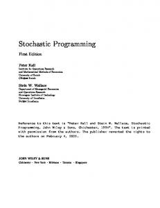
Mathematical Problems in Engineering 2.1.2. Flow Shop. In an IC packaging and testing factory, an order is often divided into several work orders. Figure 1 shows that each work order is manufactured based on the production flow. Meanwhile, IC packaging and testing factories have multiple production lines. For example, a certain large-scale domestic packaging and testing factory has approximately 25 lines. This study only investigates the bottleneck stations in these factories, namely, the DB, WB, and MD stations. It is described as a flow shop production environment. Thus, products will enter the WB station after leaving the DB station. After the products are processed in the WB station, they eventually enter the MD station. Therefore, products have sequential dependencies in the factory area. 2.1.3. Unrelated Parallel Machine. Given the rapid manner by which products are updated, process changes and equipment upgrade will compel semiconductor packaging and testing factories to frequently purchase new or different brands of machines to respond to market changes. Having different machine types and brands leads to the presence of different grades of machines in the production line, thereby resulting in the production pattern of unrelated parallel machines. When managements arrange orders, they exert effort to satisfy customer needs and meet the maximal service level. In addition, they manufacture by utilizing machines with the highest capacity. Hence, they first move the machines and allocate the proper machines in groups to avoid failure in production caused by inconsistencies in machine types. Most machines for the semiconductor packaging and testing industry are movable. For domestic IC packaging and testing factories, the number of moving machines reaches approximately 60 each month. 2.2. Capacity Planning. Karabuk and Wu [1] indicate that capacity planning can be described as an iterative process between the following two main components: (1) capacity expansion: given projected product demands, identify the required manufacturing technologies and their capacity levels to be physically expanded or outsourced through the planning period; (2) capacity configuration: determine which facility is to be configured with which technologies mix. The overall objective is to meet a revenue model based on strategic demand planning (which blends demand forecasting and proactive market development strategies). This objective can be viewed as meeting projected demands with minimized total costs. Chen et al. [2] present a capacity allocation and expansion problem of thin film transistor liquid crystal display (TFT-LCD) manufacturing in the multisite environment. The objective is to simultaneously seek an optimal capacity allocation plan and capacity expansion policy under singlestage, multigeneration, and multisite structures. Capacity allocation decides on profitable product mixes and allocated production quantities of each product group at each production site. Capacity expansion is concerned with determining the timing, types, and sizes of capacity investments, especially in the acquisition of auxiliary tools. A mixed integer linear programming (MILP) is proposed, which considers many practical characteristics. Finally, an industrial case study

Mathematical Problems in Engineering

Wafer

3

Incoming quality control

Crystal cutting

Patching

Die bond

Electroplating Wire bond

Molding

Shaping

Printing

Inspection

Bumping

Figure 1: Production flow of semiconductor packaging and testing factory.

modified from a Taiwanese TFT-LCD manufacturer is illustrated and sensitivity analysis of some influential parameters is also addressed. The foundry is an industry whose demand varies rapidly and whose manufacturing process is quite complicated. Chen et al. [3] explore issues on midterm capacity planning for an increment strategy of the number of auxiliary tools—“photo mask” to increase the flexibility of production. The related decisions include how to allocate appropriately the forecast demands of products among multiple sites and how to decide on the production quantities of products in each site after receiving customer-confirmed orders. By constructing the mathematical programming model of capacity planning, the rates of capacity utilization and customer order fulfillment are found to be effectively enhanced by adding new masks to increase production flexibility. Lin et al. [4] study strategic capacity planning problems under demand uncertainties in TFT-LCD industry. Demand forecasts are usually inaccurate and vary rapidly over time. Their research objective is to seek a capacity allocation and expansion policy that is robust to demand uncertainties. Special characteristics of TFT-LCD manufacturing systems are considered. A scenario-based two-stage stochastic programming model for strategic capacity planning under demand uncertainties is proposed. Comparing to the deterministic approach, their stochastic model significantly improves system robustness. Lin et al. [5] refer to capacity planning as the process of simultaneously implementing a robust capacity allocation plan and capacity expansion policy across multiple sites against stochastic demand. Their study constructs a stochastic dynamic programming (SDP) model with an embedded linear programming (LP) to generate a capacity planning policy as the demand in each period is revealed and updated. Numerical results are illustrated to prove the feasibility and robustness of the proposed SDP model. 2.3. Stochastic Programming. Given that demand uncertainty is considered, this paper aims to formulate a stochastic programming model for solving capacity allocation and migration planning problem. Dantzig [6] divided stochastic programming into two types: two-stage stochastic programming and multistage stochastic programming. Uribe et al. [7] indicated that the decision variable of two-stage stochastic programming consists of two types: “here and now” and “wait and see.” Here and now decision in the first stage refers to decision making when all information is unknown. Wait and

see decision in the second stage refers to decision making after all information has been fully revealed. Thus, decision variables for the two-stage stochastic programming are a dependent issue, and the results are more robust. Two-stage stochastic programming can be illustrated through a scenario tree. Figure 2 shows that the time point revealing uncertain factors is 𝑡 = 𝑘. The time point is used to divide decisions into two stages. The first-stage decision is from 𝑡 = 1 to 𝑡 = 𝑘. The results affect the decisions after 𝑡 = 𝑘 + 1. Thus, they extend many branches. Moreover, each branch represents a kind of scenario and a group of decision variables in the second stage. Listes¸ and Dekker [8] present a stochastic programming based approach by which a deterministic location model for product recovery network design may be extended to explicitly account for the uncertainties. They apply the stochastic models to a representative real case study on recycling sand from demolition waste in Netherlands. In Salema et al. [9] work, the design of a reverse distribution network is studied. A generalized model is proposed. It contemplates the design of a generic reverse logistics network where capacity limits, multiproduct management, and uncertainty on product demands and returns are considered. A mixed integer formulation is developed which is solved using standard B&B techniques. The model is applied to an illustrative case. Lee et al. [10] propose a stochastic programming based approach to account for the design of sustainable logistics network under uncertainty. A solution approach integrating the sample average approximation scheme with an importance sampling strategy is developed. A case study involving a large-scale sustainable logistics network in Asia Pacific region is presented to demonstrate the significance of the developed stochastic model. Cardona-Vald´es et al. [11] consider the design of a two-echelon production distribution network with multiple manufacturing plants, customers, and a set of candidate distribution centers. The main contribution of the study is to extend the existing literature by incorporating the demand uncertainty of customers within the distribution center location and transportation mode allocation decisions, as well as providing a network design satisfying both economical and service quality objectives of the decision-maker. In Kara and Onut [12] study, a two-stage stochastic revenue-maximization model is presented to determine a long-term strategy under uncertainty for a large-scale realworld paper recycling company. This network design problem includes optimal recycling center locations and optimal flow amounts between the nodes in the multifacility environment.

4

Mathematical Problems in Engineering

Scenario 1

Scenario 2

Scenario 3

First stage

Second stage

.

Time

t=1

t=2

···

t=k

t= k+1 t= k+2

t=T

Figure 2: Illustration of two-stage stochastic programming.

The proposed model is formulated with two-stage stochastic mixed integer and robust programming approaches. Pishvaee et al. [13] develop a stochastic programming model for an integrated forward/reverse logistics network design under uncertainty. An efficient deterministic mixed integer linear programming model is developed for integrated logistics network design to avoid the suboptimality caused by the separate design of the forward and reverse networks. Then the stochastic counterpart of the proposed MILP model is developed by using scenario-based stochastic approach. Numerical results show the power of the proposed stochastic model in handling data uncertainty. In Amin and Zhang [14], a closed-loop supply chain network is investigated which includes multiple plants, collection centers, demand markets, and products. A mixed integer linear programming (MILP) model is proposed that minimizes the total cost. The model is extended to consider environmental factors by weighed sums and 𝜀constraint methods. In addition, the impact of demand and return uncertainties on the network configuration is analyzed by scenario-based stochastic programming. Computational results show that the model can handle demand and return uncertainties, simultaneously. Ramezani et al. [15] present a stochastic multiobjective model for forward/reverse logistic network design under an uncertain environment including three echelons in forward direction (i.e., suppliers, plants, and distribution centers) and two echelons in backward direction (i.e., collection centers and disposal centers). The authors demonstrate a method to evaluate the systematic supply chain configuration maximizing the profit, customer responsiveness, and quality as objectives of the logistic network. Mohammadi Bidhandi and Rosnah [16] propose an integrated model and a modified solution method for solving supply chain network design problems under uncertainty. The stochastic supply chain network design model is provided as a two-stage stochastic programming. The main uncertain parameters are the operational costs, the customer demand, and capacity of the facilities. In the improved solution method, the sample average approximation technique is integrated with the accelerated

Benders’ decomposition approach to improvement of the mixed integer linear programming solution phase. Sazvar et al. [17] develop a stochastic mathematical model and propose a new replenishment policy in a centralized supply chain for deteriorating items. In this model, they consider inventory and transportation costs, as well as the environmental impacts under uncertain demand. The best transportation vehicles and inventory policy are determined by finding a balance between financial and environmental criteria. A linear mathematical model is developed and a numerical example from the real world is presented to demonstrate its applicability and effectiveness. Lin et al. [5] construct a stochastic dynamic programming model with an embedded linear programming to generate a capacity planning policy as the demand in each period is revealed and updated. Using the backward induction algorithm, the model considers several capacity expansion and budget constraints to determine a robust and dynamic capacity expansion policy in response to newly available demand information. Numerical results are also illustrated to prove the feasibility and robustness of the proposed SDP model compared to the traditional deterministic capacity planning model currently applied by the industry. A distributed energy system is a multi-input and multioutput energy system with substantial energy and economic and environmental benefits. The optimal design of such a complex system under energy demand and supply uncertainty poses significant challenges. Zhou et al. [18] propose a two-stage stochastic programming model for the optimal design of distributed energy systems. A two-stage decomposition based solution strategy is used to solve the optimization problem with genetic algorithm performing the search on the first-stage variables and a Monte Carlo method dealing with uncertainty in the second stage. Detailed computational results are presented and compared with those generated by a deterministic model. One of the most challenging issues for the semiconductor testing industry is how to deal with capacity planning and resource allocation simultaneously under demand and technology uncertainty. In addition, capacity planners require

Mathematical Problems in Engineering a tradeoff among the costs of resources with different processing technologies, while simultaneously considering resources to manufacture products. The study of K.-J. Wang and S.M. Wang [19] focuses on the decisions pertaining to (i) the simultaneous resource portfolio/investment and allocation plan, (ii) the most profitable orders from pending ones in each time bucket under demand and technology uncertainty, and (iii) the algorithm to efficiently solve the stochastic and mixed integer programming problem. The authors develop a constraint-satisfaction based genetic algorithm to resolve the above issues simultaneously. Dynamic programming approach is a class of optimal design tools, such as reinforcement learning. Liu et al. [20] proposed an online reinforcement learning algorithm for a class of affine multiple input and multiple output (MIMO) nonlinear discrete-time systems with unknown functions and disturbances. Liu et al. [21] addressed an adaptive fuzzy optimal control design for a class of unknown nonlinear discrete-time systems. The controlled systems are in a strictfeedback frame and contain unknown functions and nonsymmetric dead-zone. Wang et al. [22] developed a finitehorizon neurooptimal tracking control strategy for a class of discrete-time nonlinear systems. Chen et al. [23] studied an adaptive tracking control for a class of nonlinear stochastic systems with unknown functions. Tong et al. [24] proposed two adaptive fuzzy output feedback control approaches for a class of uncertain stochastic nonlinear strict-feedback systems without the measurements of the states. Previous studies have surveyed about capacity planning issue, but only a few studies have focused on the capacity allocation problem considering machine/tool migration planning and demand uncertainty simultaneously. This paper aims to determine the best capacity allocation with limited resources to achieve net profit maximization in the semiconductor packaging and testing industry. Customer demand is regarded as an uncertain parameter in formulating a twostage scenario-based stochastic programming model. This model seeks to respond to sharp demand fluctuations. Even if future demand is uncertain, migration decision for machines and tools will still obtain better robust results for various demand scenarios. Sensitivity analysis is also performed to evaluate the effect of different parameters on net profit.

3. Capacity Planning of the Semiconductor Packaging and Testing Industry 3.1. Characteristics of Capacity Planning of the Semiconductor Packaging and Testing Industry. This study aims to determine machine migration, tool migration in all production lines, resource configuration, capacity allocation, and product flow under demand uncertainty to achieve net profit maximization. 3.1.1. Resource Configuration. The manufacturing process entails that a product should sequentially go through the DB, WB, and MD stations for assembly-line production. The product considers the machine type in resource configuration during the DB and WB stages. However, three resources,

5

Product 1

Product category

Production stage

Machine type

Die bond

k1

k2

Wire bond

k2

Tool type

Material type

k3

Molding

k1

k2

n1

n2

m4

m4

Resource configuration

Figure 3: Illustration of resource configuration.

namely, machine type, tool type, and material category, are considered in the MD stage. Figure 3 shows that product 1 is manufactured in machine 𝑘1 or 𝑘2 in the DB station. This product is then processed in machine 𝑘2 or 𝑘3 in the WB station. Thereafter, the product is manufactured in the MD station through 𝑘1 + 𝑛1 + 𝑚4 or 𝑘2 + 𝑛2 + 𝑚4. 3.1.2. Product Flow. This study disregards defective products and only considers production through the three sequential stages. Moreover, product flow balance must be maintained in the production line. Hence, the total product input must equal the final total output. For example, the product input for product 1 is 1,000 units. Furthermore, 400 and 600 units are produced in lines 1 and 2, respectively. After production through the three sequential stages, the final total output remains as 1,000 units. 3.1.3. Capacity Allocation. The capacity planning of all received orders is executed based on the current existing resources in all production stages. A product is not limited to the same production line during the entire production process; that is, a product can be manufactured in the different lines through three production stages. For example, a company has two lines, if the input of product 1 is 1,000 units. Take line 1 for explanation. Firstly, 400 units are manufactured in the DB station using machine 𝑘1 and 600 units using machine 𝑘2. Thereafter, 400 units are manufactured in the WB station using machine 𝑘2 and 200 units using machine 𝑘3. Finally, 200 units are manufactured in the MD station using resource configuration 𝑘1 + 𝑛1 + 𝑚4 and 300 units using 𝑘2 + 𝑛2 + 𝑚4. Thus, 500 units of product 1 can be made after the three production stages for this product are completed sequentially in line 1. The remaining 500 units are allocated to all production stages in line 2 for manufacturing. 3.1.4. Machine and Tool Migration. The presence of several production lines and machines with different technological capability in a company will result in variations in the

6 production capacities of all lines. Machines can be moved to all lines in each production stage, and tools can be moved to all lines in the MD stage based on the total number of available machines and tools. 3.2. Mathematical Programming of Capacity Planning Problem for the Semiconductor Packaging and Testing Industry under Demand Uncertainty. A mathematical model of two-stage scenario-based stochastic programming is formulated by considering customer demand as an uncertain parameter. This study aims to respond to sharp demand fluctuation. Even if future demand is uncertain, machine and tool migration decisions are robust results for all demand scenarios. 3.2.1. Definition and Description of Capacity Planning Problem under Demand Uncertainty. This study uses a scenario tree to illustrate the uncertain factor (Figure 4). Machine and tool migration decisions are deemed to be the decisions made in the first stage. The results of these decisions remain constant with the varying customer demands. Moreover, the secondstage capacity allocation decisions must be made based on the first-stage decision results. The results in the secondstage change with the varying customer demands. In this study, two-stage decisions should be optimally determined to achieve net profit maximization. (1) First-Stage Decision: Robust Capacity Migration Decision That Considers Demand Uncertainty. Given three demand scenarios, each type of machine and tool is considered to determine when and what quantity of machines and tools are migrated between lines in the production stage. Hence, capacity migration decision must be made in advance to consider the robust decision under demand uncertainty as being unrelated to different demand scenarios. (2) Second-Stage Decision: Capacity Allocation Decision after All Demand Information Has Been Completely Revealed. The following factors are determined after a certain demand scenario occurs: (1) production quantity for each product in each line in all production stages during each period, (2) transportation quantity between the different production stages, (3) sales volume of each product in each period for each customer, and (4) customer service level. Therefore, capacity allocation decision is closely related to the demand scenario. According to the capacity migration result in the first stage, the optimal capacity allocation decision can be determined once a specific demand scenario occurs. 3.2.2. Two-Stage Stochastic Programming Model of Capacity Planning Problem. To solve the capacity planning problem under demand uncertainty, this study uses two-stage stochastic programming to construct a mathematical model. This section explains the indices, parameters, decision variables, objective function, and constraints. (1) Indices 𝑐 = customer (𝑐 = 1, 2, . . . , 𝐶). 𝑖 = product type (𝑖 = 1, 2, . . . , 𝐼). 𝑙 = production line (𝑙 = 1, 2, . . . , 𝐿).

Mathematical Problems in Engineering First stage Capacity migration decision

Second stage Capacity allocation decision Scenario 1 Demand

Scenario 2 Scenario 3

The uncertain factor is revealed

Figure 4: Diagrammatic sketch of scenario tree of the uncertain factor.

𝑠 = production stage (𝑠 = 1, 2, . . . , 𝑆). 𝑗 = resource configuration (𝑗 = 1, 2, . . . , 𝐽). 𝑚 = material type (𝑚 = 1, 2, . . . , 𝑀). 𝑘 = machine type (𝑘 = 1, 2, . . . , 𝐾). 𝑛 = tool type (𝑛 = 1, 2, . . . , 𝑁). 𝑡 = time period (𝑡 = 1, 2, . . . , 𝑇). 𝑟 = scenario number (𝑟 = 1, 2, . . . , 𝑅). (2) Parameters (I) Demand Related Parameters 𝑟 𝑑𝑒𝑖𝑐𝑡 = the demand quantity of customer 𝑐 for product 𝑖 in time 𝑡 under scenario 𝑟.

𝑝𝑟 = probability value occurring in scenario 𝑟 (∑𝑟 𝑝𝑟 = 1). 𝑝𝑟𝑖𝑐𝑡 = sales price of customer 𝑐 for product 𝑖 in time 𝑡. (II) Machine Related Parameters 𝑘𝑙𝑙𝑠𝑘 = initial amount of machine 𝑘 in line 𝑙 at stage 𝑠. 𝑘𝑢𝑙𝑠 = maximum number of machines in line 𝑙 at stage 𝑠. 𝑘𝑠𝑖𝑗𝑠𝑘 = required work hours of machine 𝑘 used at stage 𝑠 for manufacturing a unit of product 𝑖 with resource configuration 𝑗. 𝑘𝑎𝑠𝑘 = available work hours of machine 𝑘 at stage 𝑠.

𝑘𝑏𝑙𝑙󸀠 𝑠 = machine migration capability from lines 𝑙 to 𝑙󸀠 at stage 𝑠. (III) Tool Related Parameters 𝑛𝑙𝑙𝑠𝑛 = initial amount of tool 𝑛 in line 𝑙 at stage 𝑠. 𝑛𝑢𝑙𝑠 = maximum number of tools in line 𝑙 at stage 𝑠. 𝑛𝑠𝑖𝑗𝑠𝑛 = required work hours of tool 𝑛 used at stage 𝑠 for manufacturing a unit of product 𝑖 with resource configuration 𝑗. 𝑛𝑎𝑠𝑛 = available work hours of tool 𝑛 at stage 𝑠.

𝑛𝑏𝑙𝑙󸀠 𝑠 = tool migration capability from lines 𝑙 to 𝑙󸀠 at stage 𝑠.

Mathematical Problems in Engineering

7

(IV) Material Related Parameters

(3) Decision Variables

𝑚𝑞𝑠𝑚𝑡 = total available quantity of material 𝑚 at stage 𝑠 in time 𝑡. 𝑚𝑠𝑖𝑗𝑠𝑚 = consumption ratio of material 𝑚 for manufacturing a unit of product 𝑖 at stage 𝑠 with resource configuration 𝑗.

(I) First-Stage Decision Variables: Capacity Migration Decision 𝐾𝑄𝑙𝑠𝑘𝑡 = the number of machines 𝑘 for line 𝑙 at stage 𝑠 in time 𝑡. 𝐾𝑀𝑙𝑙󸀠 𝑠𝑘𝑡 = the migration number of machines 𝑘 from line 𝑙 to line 𝑙󸀠 at stage 𝑠 in time 𝑡. 𝑁𝑄𝑙𝑠𝑛𝑡 = the number of tools 𝑛 for line 𝑙 at stage 𝑠 in time 𝑡.

(V) Production Capability Related Parameter 𝑡𝑓𝑖𝑗𝑠 = production capability of product 𝑖 at stage 𝑠 with resource configuration 𝑗.

𝑁𝑀𝑙𝑙󸀠 𝑠𝑛𝑡 = the migration number of tools 𝑛 from line 𝑙 to line 𝑙󸀠 at stage 𝑠 in time 𝑡. (II) Second-Stage Decision Variables: Capacity Allocation Decision and Service Level

(VI) Transportation Related Parameter 𝑡𝑏𝑙𝑠𝑙󸀠 (𝑠+1) = transportation capability from line 𝑙 at stage 𝑠 to line 𝑙󸀠 at stage 𝑠 + 1. (VII) Cost Parameters V𝑐𝑖𝑙𝑗𝑠 = production cost for manufacturing a unit of product 𝑖 in line 𝑙 at stage 𝑠 with resource configuration 𝑗. 𝑘𝑐𝑠 = machine migration cost at stage 𝑠. 𝑛𝑐𝑠 = tool migration cost at stage 𝑠.

𝑟 = production amounts of product 𝑖 with 𝑋𝑄𝑖𝑙𝑗𝑠𝑡 resource configuration 𝑗 for line 𝑙 at stage 𝑠 in time 𝑡 under scenario 𝑟. 𝑟 𝑅𝑄𝑖𝑙𝑗𝑠𝑙 󸀠 𝑗󸀠 (𝑠+1)𝑡 = transportation amounts of product 𝑖 from line 𝑙 with resource configuration 𝑗 at stage 𝑠 to line 𝑙󸀠 with resource configuration 𝑗󸀠 at stage (𝑠 + 1) in time 𝑡 under scenario 𝑟. 𝑟 = sales amounts of product 𝑖 for customer 𝑐 in 𝑆𝑄𝑖𝑐𝑡 time 𝑡 under scenario 𝑟.

𝑆𝐿𝑟𝑐 = service level for customer 𝑐 under scenario 𝑟. (4) Objective Function. Consider the following:

Maximize { } 𝑟 𝑟 ) − ∑∑∑∑∑ (V𝑐𝑖𝑙𝑗𝑠 × 𝑋𝑄𝑖𝑙𝑗𝑠𝑡 )} − ∑∑∑∑∑ (𝑘𝑐𝑠 × 𝐾𝑀𝑙𝑙󸀠 𝑠𝑘𝑡 ) ∑𝑝𝑟 {∑∑∑ (𝑝𝑟𝑖𝑐𝑡 × 𝑆𝑄𝑖𝑐𝑡 󸀠 𝑠 𝑘 𝑡 𝑟 𝑐 𝑡 𝑖 𝑙 𝑗 𝑠 𝑡 { 𝑖 } 𝑙 𝑙

(1)

− ∑∑∑∑∑ (𝑛𝑐𝑠 × 𝑁𝑀𝑙𝑙󸀠 𝑠𝑛𝑡 ) . 𝑙 𝑙󸀠

𝑠 𝑛

𝑡

The above is the objective function of two-stage stochastic programming. It aims to obtain the optimal capacity planning decision to seek the maximization of net profit, as (1); net profit = (sales revenue − variable production cost) − machine migration cost − tool migration cost.

𝑙󸀠

+ ∑𝐾𝑀𝑙󸀠 𝑙𝑠𝑘𝑡 ∀𝑙, 𝑠, 𝑘, 𝑡,

𝐾𝑀𝑙𝑙󸀠 𝑠𝑘𝑡 ≤ 𝑀 × 𝑘𝑏𝑙𝑙󸀠 𝑠

(I) First-Stage Constraints (a) Machine Migration Balance Constraints. Consider the following:

∀𝑙, 𝑠, 𝑘,

(2)

∀𝑙, 𝑠, 𝑘, 𝑡,

(3)

𝑙󸀠

𝐾𝑄𝑙𝑠𝑘𝑡 ≤ 𝑘𝑢𝑙𝑠

(5) Constraints

𝐾𝑄𝑙𝑠𝑘0 = 𝑘𝑙𝑙𝑠𝑘

𝐾𝑄𝑙𝑠𝑘𝑡 = 𝐾𝑄𝑙𝑠𝑘(𝑡−1) − ∑𝐾𝑀𝑙𝑙󸀠 𝑠𝑘𝑡

∀𝑙, 𝑙󸀠 , 𝑠, 𝑘, 𝑡.

(4) (5)

Constraint (2) shows the initial amount of machines in lines at each production stage; and constraint (3) indicates the number of machines required for lines at production stages in every period. This number of machines in the current period is equal to the number of machines in the previous period minus the number of machines moving to other lines plus

8

Mathematical Problems in Engineering

the number of machines that migrated from other lines to this line. The total initial number of machines within the company must be equal to the total number of machines after being migrated between lines without increasing or reducing the number of machines. Constraint (4) expresses that the allocated number of machines should not be more than the available space in the shop-floor production line. In addition, constraint (5) considers if machines have capability to be migrated between lines. 𝑘𝑏𝑙𝑙󸀠 𝑠 refers to a binary parameter. 1 means machines can be migrated between production lines, and 0 means they cannot be migrated. (b) Tool Migration Balance Constraints. Consider the following: 𝑁𝑄𝑙𝑠𝑛0 = 𝑛𝑙𝑙𝑠𝑛

∀𝑙, 𝑠, 𝑛,

(6)

𝑁𝑄𝑙𝑠𝑛𝑡 = 𝑁𝑄𝑙𝑠𝑛(𝑡−1) − ∑𝑁𝑀𝑙𝑙󸀠 𝑠𝑛𝑡 𝑙󸀠

+ ∑𝑁𝑀𝑙󸀠 𝑙𝑠𝑛𝑡

∀𝑙, 𝑠, 𝑛, 𝑡,

(7)

∀𝑙, 𝑠, 𝑛, 𝑡,

𝑁𝑀𝑙𝑙󸀠 𝑠𝑛𝑡 ≤ 𝑀 × 𝑛𝑏𝑙𝑙󸀠 𝑠

(8)

∀𝑙, 𝑙󸀠 , 𝑠, 𝑛, 𝑡.

(9)

Constraint (6) shows the initial amount of tools in lines at each production stage; and constraint (7) indicates the number of tools required for lines at production stages in every period. This number of tools in the current period is equal to the number of tools in the previous period minus the number of tools moving to other lines plus the number of tools that migrated from other lines to this line. The total initial number of tools within the company must be equal to the total number of tools after being migrated between lines without increasing or reducing the number of tools. Constraint (8) expresses that the allocated number of tools should not be more than the available space in the shop-floor production line. In addition, constraint (9) considers if tools have capability to be migrated between lines. 𝑛𝑏𝑙𝑙󸀠 𝑠 refers to a binary parameter. 1 means tools can be migrated between production lines, and 0 means they cannot be migrated. (c) Domain Restriction for First-Stage Decision Variables. Consider the following:

∀𝑖, 𝑙, 𝑗, 𝑠 = 2, . . . , 𝑆, 𝑡, 𝑟.

𝑙󸀠 𝑗󸀠

(12)

Overall production and transportation must satisfy line flow balance, as shown in constraints (11) and (12). The allocated production amounts in a certain line at this stage should be equal to the total amounts that are transported from this line to all lines at the next stage. On the contrary, the total amounts that are transported from all lines at the previous stage to a certain line at the current stage should be equal to the allocated production amounts in this line. (b) Capacity Constraints. Consider the following: 𝑟 × 𝑘𝑠𝑖𝑗𝑠𝑘 ) ≤ 𝐾𝑄𝑙𝑠𝑘𝑡 × 𝑘𝑎𝑠𝑘 ∑∑ (𝑋𝑄𝑖𝑙𝑗𝑠𝑡

∀𝑙, 𝑠, 𝑘, 𝑡, 𝑟,

(13)

𝑟 × 𝑛𝑠𝑖𝑗𝑠𝑛 ) ≤ 𝑁𝑄𝑙𝑠𝑛𝑡 × 𝑛𝑎𝑠𝑛 ∑∑ (𝑋𝑄𝑖𝑙𝑗𝑠𝑡

∀𝑙, 𝑠, 𝑛, 𝑡, 𝑟.

(14)

𝑖

𝑖

𝑙󸀠

𝑁𝑄𝑙𝑠𝑛𝑡 ≤ 𝑛𝑢𝑙𝑠

𝑟 ∑∑𝑅𝑄𝑖𝑙𝑟 󸀠 𝑗󸀠 (𝑠−1)𝑙𝑗𝑠𝑡 = 𝑋𝑄𝑖𝑙𝑗𝑠𝑡

𝑗

𝑗

For capacity constraints, constraints (13) and (14) indicate that the production amounts multiplied by work hours of machines or tools consumed should not exceed the number of machines or tools multiplied by available work hours of a unit of machine or tool. In short, the sum of work hours required for each product in available machine or tool should not be more than the total available resource limit of the company. (c) Material Constraint. Consider the following: 𝑟 × 𝑚𝑠𝑖𝑗𝑠𝑚 ) ≤ 𝑚𝑞𝑠𝑚𝑡 ∑∑∑ (𝑋𝑄𝑖𝑙𝑗𝑠𝑡 𝑖

𝑙

∀𝑠, 𝑚, 𝑡, 𝑟.

𝑗

(15)

For material constraint (15), generally speaking, the amounts of materials to be consumed in the production process should not be beyond the quantity restriction of available materials. With limited resources, the production amounts multiplied by the material consumption ratio per unit will be less or equal to the total available quantity of the material. (d) Production Capability Constraint. Consider the following: 𝑟 ≤ 𝑀 × 𝑡𝑓𝑖𝑗𝑠 𝑋𝑄𝑖𝑙𝑗𝑠𝑡

∀𝑖, 𝑙, 𝑗, 𝑠, 𝑡, 𝑟.

(16)

(II) Second-Stage Constraints

For production capability, constraint (16) shows whether resource configuration of a certain product is able to be used for manufacturing this product. Due to different types of machines and tools in lines at each production stage, not all resource configurations can be used for manufacturing all kinds of products. If 𝑡𝑓𝑖𝑗𝑠 = 1, the resource configuration in the line at this stage can be used for manufacturing this type of product; on the contrary, if 𝑡𝑓𝑖𝑗𝑠 = 0, they cannot be used.

(a) Production and Transportation Balance Constraints. Consider the following:

(e) Transportation Capability Constraint. Consider the following:

𝐾𝑄𝑙𝑠𝑘𝑡 , 𝐾𝑀𝑙𝑙󸀠 𝑠𝑘𝑡 , 𝑁𝑄𝑙𝑠𝑛𝑡 , 𝑁𝑀𝑙𝑙󸀠 𝑠𝑛𝑡 ∈ integer ∀𝑙, 𝑠, 𝑘, 𝑛, 𝑡.

(10)

Constraint (10) shows the domain of variables, which indicates the characteristics of its integer variables.

𝑟 𝑅𝑄𝑖𝑙𝑗𝑠𝑙 󸀠 𝑗󸀠 (𝑠+1)𝑡 ≤ 𝑀 × 𝑡𝑏𝑙𝑠𝑙󸀠 (𝑠+1)

𝑟 𝑟 𝑋𝑄𝑖𝑙𝑗𝑠𝑡 = ∑∑𝑅𝑄𝑖𝑙𝑗𝑠𝑙 󸀠 𝑗󸀠 (𝑠+1)𝑡 𝑙󸀠 𝑗󸀠

(11) ∀𝑖, 𝑙, 𝑗, 𝑠 = 1, . . . 𝑆 − 1, 𝑡, 𝑟,

∀𝑖, 𝑙, 𝑗, 𝑠, 𝑙󸀠 , 𝑗󸀠 , 𝑡, 𝑟.

(17)

For transportation capability, constraint (17) expresses whether there is transportation capability to move products

Mathematical Problems in Engineering

9

from the current stage to the next stage. The production process is an assembly flow line environment. Thus, products are bound to go through each production stage in turn and cannot revert to a previous stage. If 𝑡𝑏𝑙𝑠𝑙󸀠 (𝑠+1) = 1, there is transportation capability to move products between stages; on the contrary, if 𝑡𝑏𝑙𝑠𝑙󸀠 (𝑠+1) = 0, it indicates that there is no transportation capability. (f) Demand Fulfillment Constraints. Consider the following: 𝑟 𝑟 = 𝑆𝑄𝑖𝑐𝑡 ∑∑𝑋𝑄𝑖𝑙𝑗𝑠𝑡 𝑙

∀𝑖, 𝑠 = 𝑆, 𝑐, 𝑡, 𝑟,

(18)

∀𝑖, 𝑐, 𝑡, 𝑟.

(19)

𝑗

𝑟 𝑟 𝑆𝑄𝑖𝑐𝑡 ≤ 𝑑𝑒𝑖𝑐𝑡

Demand fulfillment is indicated by constraints (18) and (19), respectively. Constraint (18) shows that sales volume in each scenario should be equal to the total production amounts with resource configurations in all lines. Constraint (19) expresses that the sales volume must be less or equal to the demands required by customers. (g) Service Level. Consider the following: ∑ 𝑆𝑄𝑟 𝑆𝐿𝑟𝑐 = [ 𝑖 𝑟𝑖𝑐𝑡 ] ∑𝑖 𝑑𝑒𝑖𝑐𝑡

∀𝑐, 𝑡, 𝑟.

(20)

(h) Domain Restriction for Second-Stage Decision Variables. Consider the following: ≥0 󸀠

Step 1 (generation of an initial population). This study uses PSO to determine the migration number of machines and tools among the production lines. Given the initial number of machines and tools, an initial population is generated by randomly selecting the value limited to the available maximum number of machines and tools in each line. Step 2 (calculation of the fitness values). The fitness value in this study is net profit.

Constraint (20) shows that the sales volume divided by customer demands is the service level.

𝑟 𝑟 𝑟 𝑟 , 𝑅𝑄𝑖𝑙𝑗𝑠𝑙 𝑋𝑄𝑖𝑙𝑗𝑠𝑡 󸀠 𝑗󸀠 (𝑠+1)𝑡 , 𝑆𝑄𝑖𝑐𝑡 , 𝑆𝐿 𝑐

software with the ILOG CPLEX 12.6 solver to generate the optimal production amounts of products. The results are returned to the PSO algorithm to calculate the net profit and to determine whether the termination conditions have been satisfied. This study sets the termination condition as the number of generations. The search ends when the number of generations reaches the preset number of generations. If this number is reached, then the PSO algorithm is used to yield the optimal number of machines and tools of each line to the AIMMS optimal modeling software to generate the optimal production amounts of products. Fitness values are calculated during each generation. The PSO algorithm is repeated until the termination condition is satisfied. The PSO steps are stated as follows.

󸀠

∀𝑖, 𝑙, 𝑙 , 𝑗, 𝑗 , 𝑠, 𝑡, 𝑐, 𝑟.

(21)

Constraint (21) indicates variable domain restriction. 3.2.3. Capacity Planning Problem under Demand Certainty. Different from the uncertainty model, the deterministic model does not consider demand fluctuation and only considers an average demand scenario. Appendix A (see Supplementary Material available online at http://dx.doi.org/10.1155/ 2015/741329) shows the detailed mathematical programming model that is used to compare the differences in solving results between the deterministic model and stochastic programming model. 3.3. Proposed Hybrid Approach. As the scenario number is increased, solving the scenario-based stochastic programming model becomes considerably difficult because of the computation complexity. Therefore, a hybrid approach is developed to efficiently address the proposed two-stage stochastic programming model. We apply the particle swarm optimization (PSO) method combined with the AIMMS optimal modeling software in a hybrid mechanism. First, an initial solution was generated to determine the migration number of machines and tools among the production lines. This result was entered into the AIMMS optimal modeling

Step 3 (updating the speed and position of the particle). Equations (22) and (23) are used to update the speed and position, using the following symbols: 𝑡: iteration index, 𝑡 = 1, 2, . . . , 𝑇. 𝑖: particle index, 𝑖 = 1, 2, . . . , 𝐼. 𝑑: dimension index, 𝑑 = 1, 2, . . . , 𝐷. 𝑐1 : personal best position acceleration constant. 𝑐2 : global best position acceleration constant. 𝐶𝑟(𝑛): the 𝐶𝑟 of the 𝑛 time. 𝑤(𝑡): inertia weight in the 𝑡th iteration. 𝑋𝑖𝑑 (𝑡): position of the 𝑖th particle at the 𝑑th dimension in the 𝑡th iteration. 𝑉𝑖𝑑 (𝑡): velocity of the 𝑖th particle at the 𝑑th dimension in the 𝑡th iteration. 𝑝𝑏𝑒𝑠𝑡𝑖𝑑 (𝑡): personal best position of the 𝑖th particle at the 𝑑th dimension. 𝑔𝑏𝑒𝑠𝑡𝑑 (𝑡): global best position at the 𝑑th dimension. The mathematical model is expressed as follows: 𝑉𝑖𝑑 (𝑡 + 1) = 𝑤 (𝑡) 𝑉𝑖𝑑 (𝑡) + 𝑐1 𝐶𝑟 (𝑛) (𝑝𝑏𝑒𝑠𝑡𝑖𝑑 (𝑡) − 𝑋𝑖𝑑 (𝑡))

(22)

+ 𝑐2 (1 − 𝐶𝑟 (𝑛)) (𝑔𝑏𝑒𝑠𝑡𝑖𝑑 (𝑡) − 𝑋𝑖𝑑 (𝑡)) , 𝑋𝑖𝑑 (𝑡 + 1) = 𝑋𝑖𝑑 (𝑡) + 𝑉𝑖𝑑 (𝑡 + 1) .

(23)

10

Mathematical Problems in Engineering

The following steps are used to update the individual speed and position of each dimension: (1) Set 𝑖 = 1. (2) Set 𝑑 = 1. (3) Update the 𝑑 dimension speed (𝑉𝑖𝑑 (𝑡 + 1)) in particle 𝑖 using (22). (4) Update the 𝑑 dimension position in particle 𝑖 using (23). (5) Determine whether 𝑑 is equal to 𝐷. If so, then 𝑖 = 𝑖+1. If not, then 𝑑 = 𝑑 + 1 and 𝑛 = 𝑛 + 1, and return to Step (3). (6) Determine whether 𝑖 is larger than 𝐼. If it is, this indicates that the update has concluded. If not, return to Step (2). Step 4 (updating the particle best (𝑝𝑏𝑒𝑠𝑡)). Updating the 𝑝𝑏𝑒𝑠𝑡 involves replacing the best position for current individual particles when the current individual fitness values are superior to the 𝑝𝑏𝑒𝑠𝑡 fitness values. Otherwise, the replacement is not performed and the execution is repeated until all particles have been updated. Step 5 (updating the global best (𝑔𝑏𝑒𝑠𝑡)). Updating the 𝑔𝑏𝑒𝑠𝑡 involves replacing the optimal population particles when the current optimal individual solution fitness values are superior to the 𝑔𝑏𝑒𝑠𝑡 fitness values. Otherwise, the replacement is not performed. Step 6 (determining whether the termination conditions are reached). The termination condition for the PSO algorithm presented in this study is determined when the number of iterations exceeds the set maximum iteration times. Otherwise, the process returns to Step 2.

4. Analysis and Discussion on the Semiconductor Packaging and Testing Industry Case 4.1. Introduction to the Case Background. This study aims to conduct a capacity allocation and migration planning for customer demands by considering a certain large-scale semiconductor packaging and testing factory as the case study. Three customers, eight types of products, and two production lines are involved in this case. The manufacturing process is divided into three bottleneck production stages, namely, the DB, WB, and MD stations in turn. Furthermore, the factory has three types of machines, four types of tools, and four categories of materials. The planning horizon covers four periods. For resource configuration, the DB and WB stations have three configurations consisting of machines. The MD station has seven kinds of configurations consisting of machines, tools, and materials. Appendix B (see Supplementary Material) shows the related information necessary for this case study.

4.2. Capacity Planning Results. The case problem is handled under demand uncertainty. The maximum net profit is $77,557,489.83 for the stochastic programming model. Table 1 shows the number of machines for the lines in the production stages in each time period. Table 2 presents the migration number of machines between lines in each production stage in each time period. Table 3 indicates the number of tools for the lines in the MD stage in each time period. Table 4 presents the migration number of tools between lines in the MD stage in each time period. Table 5 expresses the sales amounts of products for each customer in each time period under different scenarios. 4.3. Expected Value of Perfect Information (EVPI) and Value of the Stochastic Solution (VSS). WS stands for “wait and see”; thus the decision-maker must wait for all information to be revealed before making a decision. The objective is to maximize the net profit. The solution obtained through the deterministic model with average demand is called the expected value (EV) solution. Through the EV solution, the individual objective values of all demand scenarios can be obtained. Thereafter, these objective values are multiplied by the occurring probability of the corresponding scenario to obtain the expected value, namely, the expected result of using the EV solution (EEV). The “here and now” type indicates the maximized net profit value of stochastic programming, which is called SP. For the capacity allocation and migration planning problem in this study, the solving result through SP under uncertainty is compared with the deterministic model. Two indicators, namely, expected value of perfect information (EVPI) and value of the stochastic solution (VSS), are used for analysis. The optimal objective value of the stochastic programming model is compared with the expected value of the WS solutions. The latter is calculated by determining the optimal solution for each possible realization of the demand scenarios with certainty. Clearly, it is better to know the value of the future actual demand before making a decision than having to make the decision before knowing. The difference between these two expected objective values is called EVPI. Furthermore, EVPI measures the maximum amount a decision-maker would be willing to pay in return for complete (and accurate) information about the future to solve uncertainty. Thus, EVPI is defined in (24). If EVPI is smaller, the stochastic programming result is closer to the result obtained with complete information. By contrast, if EVPI is larger, the influence of uncertain factors is greater and the price paid for obtaining complete information is considerably high: EVPI = WS − SP.

(24)

VSS is used to measure the ability of the stochastic programming model to increase net profit, with the attempt to solve uncertain factors. It is the difference between the solution of the SP model and the expected value of the objective function when fixing parameters to average values and using the corresponding optimal solution. Thus, VSS is defined in (25). VSS conveys to us how much we can gain

Mathematical Problems in Engineering

11

Table 1: The number of machines for lines at production stages in each time period (𝐾𝑄𝑙𝑠𝑘𝑡 ).

Line

Production stage 1 10 5 9 0 0 2

DB WB MD DB WB MD

𝑙1

𝑙2

𝑘1 Time (month) 2 3 10 10 4 4 9 9 0 0 0 0 2 2

4 10 4 9 0 0 2

1 15 6 10 5 10 5

Types of machine 𝑘2 Time (month) 2 3 15 15 6 6 10 10 5 5 10 10 5 5

4 15 6 10 5 10 5

1 0 1 1 6 8 6

𝑘3 Time (month) 2 3 0 0 1 1 1 1 6 6 8 8 6 6

4 0 1 1 6 8 1

Table 2: The migration number of machines between lines at each production stage in each time period (𝐾𝑀𝑙𝑙󸀠 𝑠𝑘𝑡 ).

Line Move to line

𝑙1 𝑙2

𝑙2 𝑙1

DB Types of machine 𝑘2 Time 4 1 2 3 4 1 0 0 0 0 0 0 0 0 0 0 0 0

𝑘1 Time 1 2 3 0 0 0 0 0 0

𝑘3 𝑘1 Time Time 2 3 4 1 2 3 0 0 0 0 1 0 0 0 0 0 0 0

Production stage WB Types of machine 𝑘2 Time 4 1 2 3 4 1 0 0 0 0 0 0 0 0 0 0 0 1

𝑘3 𝑘1 Time Time 2 3 4 1 2 3 0 0 0 1 0 0 0 0 0 0 0 0

MD Types of machine 𝑘2 Time 4 1 2 3 4 1 0 0 0 0 0 0 0 0 0 0 0 2

𝑘3 Time 2 3 4 0 0 0 0 0 0

Table 3: The number of tools for lines at MD stage in each time period (𝑁𝑄𝑙𝑠𝑛𝑡 ).

Line 𝑙1 𝑙2

Production stage

MD MD

𝑛1 Time (month) 1 2 3 4 1 1 1 1 29 29 29 29

Types of tool 𝑛2 𝑛3 Time (month) Time (month) 1 2 3 4 1 2 3 4 30 29 29 29 1 1 1 1 0 1 1 1 19 19 19 19

𝑛4 Time (month) 1 2 3 4 29 29 29 29 1 1 1 1

Table 4: The migration number of tools between lines at MD stage in each time period (𝑁𝑀𝑙𝑙󸀠 𝑠𝑛𝑡 ). Types of tool Line 𝑙1 𝑙2

𝑛1 Time

Move to line 𝑙2 𝑙1

1 0 1

2 0 0

𝑛2 Time 3 0 0

4 0 0

1 0 0

2 1 0

more if SP is used. If VSS is larger, the SP result is better than the expected result when using the EV solution obtained by replacing all possible demands with their average values: VSS = SP − EEV.

(25)

The related measurements for the case problem in this study are showed in Table 6. 4.3.1. Net Profit Fluctuation under Different Combinations of Probability. Different probability combinations are designed to investigate whether the occurring probability of all

𝑛3 Time 3 0 0

4 0 0

1 0 1

2 0 0

𝑛4 Time 3 0 0

4 0 0

1 1 0

2 0 0

3 0 0

4 0 0

demand scenarios affects the net profit. The combined design individually provides significantly high probability values to low, mean, and high demand scenarios. Table 7 shows that the capacity planning results under all probability combinations indicate that net profits using the SP model are higher than those using the deterministic model. Moreover, if the occurring probability of low demand scenario is 0.8, then its net profit is significantly lower than that of the mean demand or high demand scenario, which possesses an occurring probability of 0.8. Therefore, the occurring probability of the scenario is positively related to the demand of each

12

Mathematical Problems in Engineering Table 5: The sales amounts of products for each customer in each time period under different scenarios (𝑆𝑄𝑟𝑖𝑐𝑡 ).

Scenario Scenario 1 Scenario 1 Scenario 1 Scenario 1 Scenario 1 Scenario 1 Scenario 1 Scenario 1 Scenario 2 Scenario 2 Scenario 2 Scenario 2 Scenario 2 Scenario 2 Scenario 2 Scenario 2 Scenario 3 Scenario 3 Scenario 3 Scenario 3 Scenario 3 Scenario 3 Scenario 3 Scenario 3

Product

Customer

𝑖1 𝑖2 𝑖3 𝑖4 𝑖5 𝑖6 𝑖7 𝑖8 𝑖1 𝑖2 𝑖3 𝑖4 𝑖5 𝑖6 𝑖7 𝑖8 𝑖1 𝑖2 𝑖3 𝑖4 𝑖5 𝑖6 𝑖7 𝑖8

𝑐1 𝑐1 𝑐1 𝑐2 𝑐2 𝑐3 𝑐3 𝑐3 𝑐1 𝑐1 𝑐1 𝑐2 𝑐2 𝑐3 𝑐3 𝑐3 𝑐1 𝑐1 𝑐1 𝑐2 𝑐2 𝑐3 𝑐3 𝑐3

1 45,955 137,866 99,999 91,911 22,978 99,999 53,614 199,998 48,000 144,000 99,999 96,000 24,000 99,999 56,000 199,998 50,045 150,134 58,416 100,089 25,022 99,999 58,386 199,998

Table 6: The related measurements for the case problem.

WS SP EEV EVPI VSS VSS × 100 (%) EEV

Net profit 77,560,489.83 77,557,489.83 77,439,044.28 3000.00 118,445.55 0.15%

corresponding scenario; that is, determining the occurring probability of scenario is highly important when using the SP model. 4.3.2. Changes in EVPI and VSS under Different Probability Combinations. The current study analyzes whether the occurring probabilities of all demand scenarios have an effect on EVPI and VSS. Accordingly, several probability combinations of demand scenarios are designed, including the probability combination with considerably high occurring probability of specific demand scenario. EVPI and VSS under different probability combinations are shown in Table 8. Figure 5 shows that when the probability combination is (0.1, 0.1, 0.8), the net profit gap between the deterministic model and SP model is $50,569. Moreover, the decision-maker is

Time period (month) 2 3 80,375 11,400 40,188 72,154 21,265 0 60,281 54,115 120,563 45,096 48,893 0 24,113 53,175 21,768 0 96,000 13,500 48,000 96,000 22,857 0 72,000 72,000 144,000 60,000 54,307 48,647 28,800 68,192 26,000 0 108,987 0 55,812 116,115 0 0 83,719 89,885 167,437 74,904 58,778 0 33,487 82,200 30,232 0

4 37,666 0 62,030 0 15,066 33,379 33,899 11,300 60,000 0 96,428 0 24,000 0 54,000 18,000 82,334 0 99,999 0 32,934 61,055 74,101 24,700

Table 7: The related measurements for different probability combinations. Probability combination∗

WS

SP

EEV

(0.8, 0.1, 0.1) (0.1, 0.8, 0.1) (0.1, 0.1, 0.8)

69,966,361.66 78,027,716.20 84,687,393.96

69,962,311.66 78,023,666.20 84,686,493.96

69,959,928.00 78,021,282.53 84,635,924.63

∗

The occurring probability of low demand, mean demand, and high demand scenarios, respectively.

willing to pay $900 in return for the complete information on future uncertainty. Hence, when the occurring probability of high demand is higher, EVPI is lower. Specifically, the solving result of net profit under complete (perfect) information is closer to the decision made by the SP model. Similarly, if VSS is higher, then the obtained benefit from the SP model is better. 4.3.3. Effect of Demand Variability on Net Profit, EVPI, and VSS. Three types of demand variability are designed in this study. Base Case aims to infer demands of all scenarios using the coefficient of variation. Small variation is equal to 90% of Base Case (middle variation), and large variation is 110% of Base Case. After individually solving the three different variations, the net profit in all variations under the SP model

Mathematical Problems in Engineering

13

Table 8: EVPI and VSS under different probability combinations. EVPI 4,050 3,600 3,150 3,000 2,250 900

VSS 2,384 9,267 16,151 18,446 29,918 50,569

∗

The occurring probability of low demand, mean demand, and high demand scenarios, respectively.

Demand variability Small variation Middle variation Large variation

EEV 72,884,515 77,539,044 82,113,557

SP 72,888,460 77,557,489 82,134,434

Gap 3,945 18,445 20,877

25,000 20,000 15,000 10,000 5,000 0

Small variation

Middle variation

Large variation

(0.1, 0.1, 0.8)

(0.2, 0.3, 0.5)

(0.333, 0.333, 0.333)

(0.3, 0.4, 0.3)

(0.3, 0.5, 0.2)

Gap in net profit between EEV and SP (0.8, 0.1, 0.1)

60000 50000 40000 30000 20000 10000 0

Table 9: Comparison of net profit under demand variability.

Gap in net profit

Probability combinations (0.8,0.1,0.1) (0.3,0.5,0.2) (0.3,0.4,0.3) (0.333,0.333,0.333) (0.2,0.3,0.5) (0.1,0.1,0.8)

∗

Probability combinations (low/mean/high demand) EVPI VSS

Figure 5: The diagram for EVPI and VSS under different probability combinations.

and deterministic model can be calculated (Table 9). It also can be found from Figure 6 that the gap in net profit will increase with the increase of demand variation. Thus, the SP model considers demand uncertainty, and its result is better than that of the deterministic model, which only considers average demand. 4.4. Sensitivity Analysis 4.4.1. Effect of Demand Change on Machine and Tool Migration and Net Profit. Demand change is the primary problem discussed in this study. The semiconductor packaging and testing industry cannot accurately forecast the actual demand of customers. If the demand change constantly shows positive growth or a substantial negative reduction, then the twostage SP model will significantly respond to considerable demand change compared to the deterministic model. Hence, when the actual demand is lower, capacity waste can be reduced. By contrast, when the actual demand is higher, capacity shortage can be avoided. For the case company in this study, the increasing demand results in the continuous improvement in net profit because of the demand growth. However, the number of machine and tool migrations is unaffected by demand change; as demand decreases, net profit and the number of machine and tool migrations are reduced as demand is decreased. Doing so can avoid unnecessary migration costs, as shown in Tables 10 and 11.

Figure 6: Gap in net profit under different demand variability.

4.4.2.Effect of Changes in Unit Migration Cost on Machine/Tool Migration and Net Profit. The unit migration cost affects moving times. When the unit migration cost is more expensive, it significantly increases the total migration cost, thereby lowering the net profit. When the unit migration cost is considerably inexpensive, frequent machine/tool migrations and production amounts of products may increase, thereby increasing the net profit. For the case company in this study, when the unit migration cost starts to increase, the net profit will decrease, and the number of machine/tool migrations will also decrease. When the unit migration cost is down, the net profit will increase. However, the number of machine/tool migrations remains constant, as shown in Tables 12 and 13. 4.4.3. Effect of Sales Price Fluctuation on Machine and Tool Migration and Net Profit. The sales price of products affects net profit. If sales price is higher, then the net profit increases. By contrast, if sale price is down, then the net profit decreases. When sales price is higher, salesmen will attempt to address the customer needs and provide higher service level; when sales price is lower, they cannot completely meet the customer promise needs, thereby resulting in the occurrence of short supply, which lowers service level. Thus, a better balanced decision must be determined between sales revenue and production/migration costs. For the case company in this study, as shown in Tables 14 and 15, when sales price is raised, the net profit increases and machine/tool migration decisions are not affected; on the contrary, when the sales price is lowered, the net profit decreases and machine/tool migration amounts are also reduced because of low sales price. 4.4.4. Effect of Migration Capability on Machine and Tool Migration and Net Profit. Given that capacity allocation decisions are made, several products may not be manufactured because of the limited flexibility of machine and tool migration. Production capacity cannot be allocated

14

Mathematical Problems in Engineering Table 10: Changes in migration costs and net profit under positively growing demand.

2 13,000 4,000 110,214,963

Machine migration cost Tool migration cost Net profit

4 13,000 4,000 136,961,643

Demand growth multiples 6 13,000 4,000 141,816,636

8 13,000 4,000 145,421,413

10 13,000 4,000 146,009,670

Table 11: Changes in migration costs and net profit under negatively decreasing demand.

Machine migration cost Tool migration cost Net profit

0.9 9,500 3,000 72,888,460

0.7 6,500 3,000 58,776,998

Demand reduction multiples 0.5 6,500 1,000 42,229,098

0.3 6,500 1,000 25,345,259

0.1 6,500 1,000 8,443,419

Table 12: Changes in migration decisions and net profit under the increased unit migration cost.

Machine migration amount Tool migration amount Net profit

2 5 4 77,543,489

Increased unit migration cost (multiple) 5 10 50 4 4 3 4 3 3 77,505,527 77,454,535 77,073,544

100 3 2 76,645,716

Table 13: Changes in migration decisions and net profit under the reduced unit migration cost.

Machine migration amount Tool migration amount Net profit

0.9 5 4 77,558,889

Reduced unit migration cost (multiple) 0.7 0.5 0.3 5 5 5 4 4 4 77,561,689 77,564,489 77,567,289

flexibly between different production lines. Without migration capability limitation, all machines and tools become movable, which is advantageous to the adjustment of capacity. By contrast, if the flexibility of migration is limited, then adjusting to a considerably high capacity level is difficult, thereby decreasing net profit, as shown in Table 16. Moreover, the number of machine migrations increases as migration flexibility opens.

5. Conclusion This study considers a certain large-scale semiconductor packaging and testing factory to address capacity allocation and migration planning problems under demand uncertainty. The planning scope includes three bottleneck stations, namely, the DB, WB, and MD stations. Moreover, the twostage stochastic programming approach is applied and its mathematical model is formulated to solve this problem. Machine and tool migration decisions are deemed to be the first-stage decision. The second-stage decision is capacity

0.1 5 4 77,570,089

allocation, which can be solved once the uncertain factors are revealed. Hence, when demand is changed, machine and tool migration decisions remain to be a better robust result. The measuring indicators, EVPI and VSS, are applied to evaluate the SP model and the deterministic EEV model. SP obtains a better net profit than EEV; the VSS values obtained are positive. Thus, the two-stage SP model proposed in this study can indeed improve the deficiencies of the traditional deterministic model. Furthermore, decision-makers can make good use of sensitivity analysis results as reference. This paper can assist the semiconductor packaging and testing factory in simultaneously conducting capacity allocation and resource configuration planning with the use of existing resources. Moreover, the two-stage SP method determines a robust machine and tool migration decision in advance as a response to future fluctuating demand. This model can also obtain the optimal capacity allocation and migration planning decision. It is closer to actual industry application and reaches the economic target of semiconductor packaging and testing industry, namely, meeting customer needs and maximizing net profit.

Mathematical Problems in Engineering

15

Table 14: Changes in migration decisions and net profit under the increased sales price.

Machine migration amount Tool migration amount Net profit

2 5 4 220,928,485

Increased sales price (multiple) 6 10 5 5 4 4 514,230,084 863,568,161

4 5 4 339,561,046

50 5 4 4,356,948,922

Table 15: Changes in migration decisions and net profit under the reduced sales price.

Machine migration amount Tool migration amount Net profit

0.9 5 4 68,824,037

0.7 5 4 51,357,134

Increased sales price (multiple) 0.5 0.3 5 5 4 4 33,890,230 16,423,326

Table 16: Changes in migration decisions and net profit under different migration flexibility.

Machine migration amount Tool migration amount Machine migration cost Tool migration cost Net profit

Migration capability Limited Opened 3 6 3 3 6,500 11,500 3,000 3,000 78,227,955 84,600,698

Conflict of Interests

[8]

[9]

[10]

[11]

The authors declare that there is no conflict of interests regarding the publication of this paper.

References [1] S. Karabuk and S. D. Wu, “Coordinating strategic capacity planning in the semiconductor industry,” Operations Research, vol. 51, no. 6, pp. 839–849, 2003. [2] T.-L. Chen, Y.-Y. Chen, and H.-C. Lu, “A capacity allocation and expansion model for TFT-LCD multi-site manufacturing,” Journal of Intelligent Manufacturing, vol. 24, no. 4, pp. 847–872, 2013. [3] Y.-Y. Chen, T.-L. Chen, and C.-D. Liou, “Medium-term multiplant capacity planning problems considering auxiliary tools for the semiconductor foundry,” International Journal of Advanced Manufacturing Technology, vol. 64, no. 9-12, pp. 1213–1230, 2013. [4] J. T. Lin, C.-H. Wu, T.-L. Chen, and S.-H. Shih, “A stochastic programming model for strategic capacity planning in thin film transistor-liquid crystal display (TFT-LCD) industry,” Computers and Operations Research, vol. 38, no. 7, pp. 992–1007, 2011. [5] J. T. Lin, T.-L. Chen, and H.-C. Chu, “A stochastic dynamic programming approach for multi-site capacity planning in TFTLCD manufacturing under demand uncertainty,” International Journal of Production Economics, vol. 148, pp. 21–36, 2014. [6] G. B. Dantzig, “Linear programming under uncertainty,” Management Science, vol. 1, pp. 197–206, 1955. [7] A. M. Uribe, J. K. Cochran, and D. L. Shunk, “Two-stage simulation optimization for agile manufacturing capacity planning,”

[12]

[13]

[14]

[15]

[16]

[17]

0.1 3 2 1,499,394

International Journal of Production Research, vol. 41, no. 6, pp. 1181–1197, 2003. O. Listes¸ and R. Dekker, “A stochastic approach to a case study for product recovery network design,” European Journal of Operational Research, vol. 160, no. 1, pp. 268–287, 2005. M. I. G. Salema, A. P. Barbosa-Povoa, and A. Q. Novais, “An optimization model for the design of a capacitated multiproduct reverse logistics network with uncertainty,” European Journal of Operational Research, vol. 179, no. 3, pp. 1063–1077, 2007. D.-H. Lee, M. Dong, and W. Bian, “The design of sustainable logistics network under uncertainty,” International Journal of Production Economics, vol. 128, no. 1, pp. 159–166, 2010. ´ Y. Cardona-Vald´es, A. Alvarez, and D. Ozdemir, “A bi-objective supply chain design problem with uncertainty,” Transportation Research Part C: Emerging Technologies, vol. 19, no. 5, pp. 821– 832, 2011. S. S. Kara and S. Onut, “A two-stage stochastic and robust programming approach to strategic planning of a reverse supply network: the case of paper recycling,” Expert Systems with Applications, vol. 37, no. 9, pp. 6129–6137, 2010. M. S. Pishvaee, F. Jolai, and J. Razmi, “A stochastic optimization model for integrated forward/reverse logistics network design,” Journal of Manufacturing Systems, vol. 28, no. 4, pp. 107–114, 2009. S. H. Amin and G. Zhang, “A multi-objective facility location model for closed-loop supply chain network under uncertain demand and return,” Applied Mathematical Modelling, vol. 37, no. 6, pp. 4165–4176, 2013. M. Ramezani, M. Bashiri, and R. Tavakkoli-Moghaddam, “A new multi-objective stochastic model for a forward/reverse logistic network design with responsiveness and quality level,” Applied Mathematical Modelling, vol. 37, no. 1-2, pp. 328–344, 2013. H. Mohammadi Bidhandi and M. Y. Rosnah, “Integrated supply chain planning under uncertainty using an improved stochastic approach,” Applied Mathematical Modelling, vol. 35, no. 6, pp. 2618–2630, 2011. Z. Sazvar, S. M. J. M. Al-E-Hashem, A. Baboli, and M. R. A. Jokar, “A bi-objective stochastic programming model for a centralized green supply chain with deteriorating products,” International Journal of Production Economics, vol. 150, pp. 140– 154, 2014.

16 [18] Z. Zhou, J. Zhang, P. Liu, Z. Li, M. C. Georgiadis, and E. N. Pistikopoulos, “A two-stage stochastic programming model for the optimal design of distributed energy systems,” Applied Energy, vol. 103, pp. 135–144, 2013. [19] K.-J. Wang and S.-M. Wang, “Simultaneous resource portfolio planning under demand and technology uncertainty in the semiconductor testing industry,” Robotics and ComputerIntegrated Manufacturing, vol. 29, no. 5, pp. 278–287, 2013. [20] Y. J. Liu, T. Li, S. C. Tong, C. L. P. Chen, and D. J. Li, “Reinforcement learning design-based adaptive tracking control with less learning parameters for nonlinear discrete-time MIMO systems,” IEEE Transactions on Neural Networks and Learning Systems, vol. 26, pp. 165–176, 2015. [21] Y.-J. Liu, Y. Gao, S. Tong, and Y. Li, “Fuzzy approximation-based adaptive backstepping optimal control for a class of nonlinear discrete-time systems with dead-zone,” IEEE Transactions on Fuzzy Systems, 1 page, 2015. [22] D. Wang, D. Liu, and Q. Wei, “Finite-horizon neuro-optimal tracking control for a class of discrete-time nonlinear systems using adaptive dynamic programming approach,” Neurocomputing, vol. 78, no. 1, pp. 14–22, 2012. [23] C. L. P. Chen, Y.-J. Liu, and G.-X. Wen, “Fuzzy neural networkbased adaptive control for a class of uncertain nonlinear stochastic systems,” IEEE Transactions on Cybernetics, vol. 44, no. 5, pp. 583–593, 2014. [24] S. C. Tong, Y. Li, Y. M. Li, and Y. J. Liu, “Observer-based adaptive fuzzy backstepping control for a class of stochastic nonlinear strict-feedback systems,” IEEE Transactions on Systems, Man, and Cybernetics, Part B: Cybernetics, vol. 41, no. 6, pp. 1693–1704, 2011.

Mathematical Problems in Engineering

Advances in

Operations Research Hindawi Publishing Corporation http://www.hindawi.com

Volume 2014

Advances in

Decision Sciences Hindawi Publishing Corporation http://www.hindawi.com

Volume 2014

Journal of

Applied Mathematics

Algebra

Hindawi Publishing Corporation http://www.hindawi.com

Hindawi Publishing Corporation http://www.hindawi.com

Volume 2014

Journal of

Probability and Statistics Volume 2014

The Scientific World Journal Hindawi Publishing Corporation http://www.hindawi.com

Hindawi Publishing Corporation http://www.hindawi.com

Volume 2014

International Journal of

Differential Equations Hindawi Publishing Corporation http://www.hindawi.com

Volume 2014

Volume 2014

Submit your manuscripts at http://www.hindawi.com International Journal of

Advances in

Combinatorics Hindawi Publishing Corporation http://www.hindawi.com

Mathematical Physics Hindawi Publishing Corporation http://www.hindawi.com

Volume 2014

Journal of

Complex Analysis Hindawi Publishing Corporation http://www.hindawi.com

Volume 2014

International Journal of Mathematics and Mathematical Sciences

Mathematical Problems in Engineering

Journal of

Mathematics Hindawi Publishing Corporation http://www.hindawi.com

Volume 2014

Hindawi Publishing Corporation http://www.hindawi.com

Volume 2014

Volume 2014

Hindawi Publishing Corporation http://www.hindawi.com

Volume 2014

Discrete Mathematics

Journal of

Volume 2014

Hindawi Publishing Corporation http://www.hindawi.com

Discrete Dynamics in Nature and Society

Journal of

Function Spaces Hindawi Publishing Corporation http://www.hindawi.com

Abstract and Applied Analysis

Volume 2014

Hindawi Publishing Corporation http://www.hindawi.com

Volume 2014

Hindawi Publishing Corporation http://www.hindawi.com

Volume 2014

International Journal of

Journal of

Stochastic Analysis

Optimization

Hindawi Publishing Corporation http://www.hindawi.com

Hindawi Publishing Corporation http://www.hindawi.com

Volume 2014

Volume 2014