Solving Two-Stage Stochastic Programming ... - Semantic Scholar

Solving Two-Stage Stochastic Programming Problems with Level Decomposition Csaba I. Fábián∗

Zoltán Sz˝oke†

Abstract We propose a new variant of the two-stage recourse model. It can be used e.g., in managing resources in whose supply random interruptions may occur. Oil and natural gas are examples for such resources. Constraints in the resulting stochastic programming problems can be regarded as generalizations of integrated chance constraints. For the solution of such problems, we propose a new decomposition method that integrates a bundletype convex programming method with the classic distribution approximation schemes. Feasibility and optimality issues are taken into consideration simultaneously, since we use a convex programming method suited for constrained optimization. This approach can also be applied to traditional two-stage problems whose recourse functions can be extended to the whole space in a computationally efficient way. Network recourse problems are an example for such problems. We report encouraging test results with the new method.

Keywords Stochastic recourse models – Decomposition – Successive approximation. Mathematics Subject Classification

90C15 Stochastic programming.

Introduction In this paper, we identify classes of two-stage recourse problems where the expected recourse function can be extended to the whole space in a computationally efficient way. Network recourse problems constitute such a problem class. Two-stage recourse problems belonging to such classes can be formulated as constrained convex programming problems. This formulation is called standard model in the paper. We also propose a new variant of the two-stage recourse model. Called relaxed model in the paper, this can be regarded as a generalization of the well-known integrated chance constrained model of Klein Haneveld (1986). We also give economic interpretations of the relaxed model. One of them substantially differs from traditional two-stage recourse models. It deals with the design and operation of a system that consumes certain resources in whose supply random interruptions may occur. For the above models, we propose a new solution method that we call Level Decomposition. The method consists of two known components: – The first component is an approximative version of the Constrained Level Method of Lemaréchal, Nemirovskii, and Nesterov (1995). The approximative method was proposed by Fábián (2000). – The second component involves the classic discretization and bounding methods worked out by Kall (1980), Kall and Stoyan (1982), and Birge and Wets (1986). ∗ Department of Operations Research, Lor´ and E¨ otv¨ os University of Budapest. P.O.Box 120, Budapest, H-1518 Hungary. E-mail: [email protected]. † Doctoral School in Applied Mathematics, Lor´ and E¨ otv¨ os University of Budapest.

1

The novelty of Level Decomposition is the way these two components are integrated, and the fact that the master problem is solved by a convex programming method suited for constrained optimization. In a typical implementation of the traditional solution framework, the main module is the distribution approximation scheme, and the submodule is the two-stage stochastic problem solver. To what extent the approximation should be refined between solver calls, is a difficult question, to which Mayer (1998) proposed a heuristic method. In Level Decomposition, the main module is the solver, and the approximating coarse distributions are refined in accordance with the solution process of the master problem. Using a convex programming method suited for constrained optimization means that feasibility and optimality issues are taken into consideration simultaneously. The bundle-type regularization extends to both feasibility and optimality issues. We avoid feasibility cuts that are constituents of the Benders family of solution methods. We report encouraging test results with Level Decomposition. The paper is organized as follows: In the remaining part of this section we outline the traditional two-stage recourse model, and the classic decomposition methods used for its solution. Section 1 formulates two-stage recourse models and new variants. Section 2 describes the inexact convex programming method to be used in the decomposition. Section 3 gives an algorithmic description of Level Decomposition. Section 4 deals with implementation issues. Test problems are described and parameter settings specified in Section 5. Test results are reported in Section 6. The results of the paper are summarized and potential fields of application are suggested in Section 7. The models and the solution method proposed in this paper were worked out by the first author. The method was implemented and tested with joint effort of the authors.

The traditional two-stage recourse model and the classic decomposition methods Two-stage stochastic programming problems derive from such models where decisions are made in two stages and the observation of some random event takes place in between. Hence the first decision must be made when the outcome of the random event is not yet known. For example, the first stage may represent the decision on the design of a system ; and the second stage, a decision on the operation of the system under certain circumstances. The aim may be to find a balance between investment cost and long-term operation costs. Comprehensive treatment of these models and their solution methods can be found in Kall and Wallace (1994), Prékopa (1995), Birge and Louveaux (1997), Mayer (1998), Ruszczy´ nski and Shapiro (2003), and Kall and Mayer (2005). In case the random parameters do not have a finite distribution, discretization methods are applied to make the problem tractable for solvers. Description of these methods can be found in the above mentioned books, a practical and comprehensive one in Mayer (1998). Although these methods were originally devised for the discrete approximation of a continuous distribution, they can as well be applied to approximate a discrete distribution with a coarser one. Mayer successfully applied discretization methods for this purpose. In the context of discrete finite distributions, the possible outcomes of the random events are called scenarios. In this paper we consider linear models. There are two traditional ways of formulating the problem as a mathematical programming problem: (a)

as a linear programming problem of a specific structure: For each scenario, a subproblem is included that describes the second-stage decision in case this scenario realizes. These subproblems are called recourse problems. The subproblems are linked by the first-stage variables, i.e., the variables representing the first-stage decision.

(b)

as a convex programming problem on the first-stage variables. Recourse problems are not explicitly included, but feasibility of the recourse problems is enforced by cuts on the feasible region. The objective function is not known explicitly, but supporting hyperplanes can be constructed to its graph. 2

The above two formulations are equivalent from a mathematical point of view. They only differ in that they suggest (apparently) different solution approaches. Dantzig and Madansky (1961) observed that the dual of the linear programming problem (a) fits the prototype for the Dantzig-Wolfe decomposition (1960). Based on the convex programming (b) formulation, Van Slyke and Wets (1969) worked out a cutting-plane method called L-Shaped Method. It turned out to be the same as the Benders decomposition method (1962), specialized for the linear programming problem (a). Hence the L-Shaped Method on the one hand, and the Dantzig-Wolfe decomposition applied to the dual of the problem (a) on the other hand, are identical methods. The cutting-plane formulation has the advantage that it gives a clear visual impression of the procedure. In their pure forms, decomposition or cutting-plane methods are impractical: they are known to be unstable, the convergence is slow, and hence the number of the master iterations is large. Implementations must deal with a constantly growing master problem. (There is no effective constraint reduction strategy, because the master problem tends to be dual degenerate.) Several stochastic programming decomposition methods were proposed to improve efficiency. Practical descriptions can be found in Mayer (1998), Ruszczy´ nski (2003), and in Kall and Mayer (2005). The Regularized Decomposition Method of Ruszczy´ nski (1986) successfully mitigates the above mentioned difficulties. It is a bundle-type method for the minimization of the sum of polyhedral convex functions over a convex polyhedron. The bundle-type penalty term in the objective function of the master problem stabilizes the procedure, and decreases the number of the iterations required. Moreover, this method lays an emphasis on keeping the master problem of a tractable size. The penalty term in the objective function eliminates dual degeneracy, and enables an effective constraint reduction strategy. In the Regularized Decomposition Method, feasibility of the solution is attained by imposing explicit constraints on the first-stage variables. These constraints, called feasibility cuts, are constituents of the Benders family of decomposition methods. Imposing feasibility cuts may cause the scope of optimization to alternate between minimizing the objective function and finding a solution that satisfies existing cuts. Implementation strategies of the Regularized Decomposition (RD) Method for two-stage stochastic prob´ etanowski (1997). They implemented the method, and solved lems are described by Ruszczy´ nski and Swi¸ several problems, each with a growing scenario set. Their test results show that the number of the RD master iterations required is a slowly increasing function of the number of the scenarios. Inexact cuts represent another possibility of improvement on pure-form decomposition methods. Inexact cuts were used by Szántai (1988) in a heuristic scheme for the solution of probabilistic constrained stochastic programming problems. For two-stage stochastic programming problems with relatively complete recourse, an inexact cut method was proposed by Zakeri, Philpott, and Ryan (2000). (Relatively complete recourse means that no extra action is needed to enforce feasibility of the recourse problems.) Before starting the procedure, they choose a decreasing sequence of tolerances which converges to 0. In the ith iteration, the inexact cut is generated with a tolerance not larger then the ith element in the pre-set sequence. Zakeri, Philpott, and Ryan report substantial improvements over the exact (pure) decomposition method. They did not apply any distribution approximation scheme. Accuracy of the cuts was regulated through decreasing the stopping tolerance for the linear programming solver used for solving the recourse problems.

1

New variants of two-stage recourse models

The first-stage and second-stage decision vectors will be denoted by x ∈ IRn and y ∈ IRs , respectively. The random event will be represented by the random vector ξ. Realizations of ξ will be denoted by ξω (ω ∈ Ω). Formally, (Ω, A, P ) is a probability space. The probability distribution can be either continuous or discrete. There are two optimization problems to be solved. The second-stage problem or recourse problem is formulated by assuming that the first-stage decision has been made, and the random event has been observed.

3

Supposing that the realization ξ ω has occurred (ω ∈ Ω), the recourse problem is min q T y subject to Tω x + W y = dω , y ≥ 0,

(1)

where q ∈ IRs , dω ∈ IRr are given vectors, and Tω ∈ IRr×n , W ∈ IRr×s are given matrices. Formally, d is a random vector, T is a random matrix ; and the random vector ξ consists of the components of d and T . Having fixed ω ∈ Ω, let Kω denote the set of those x vectors for which the recourse problem (1) is feasible. This is a convex polyhedron that we assume to be nonempty. For x ∈ Kω , let f (x, ξω ) denote the optimal objective value of the recourse problem (1). We assume that f (x, ξω ) > −∞ (x ∈ Kω ). Or equivalently, we assume that the dual of the recourse problem is feasible: max z T (dω − Tω x) subject to zT W ≤ qT .

(2)

Feasibility of the dual problem does not depend on x or ξ. The function f ( . , ξω ) : Kω → IR is a polyhedral (i.e., piecewise linear) convex function. Customary formulation prescribes that the second-stage T problems should be feasible for any realization of ξ. Formally, x should belong to the convex set K := ω∈Ω Kω . If the distribution is discrete finite then K is a polyhedron. The customary formulation of the first-stage problem that represents the first decision, is as follows: min cT x + IE (f (x, ξ)) subject to (3) Ax = b, x ≥ 0, x ∈ K, where c ∈ IRn , b ∈ IRm are given vectors, and A ∈ IRm×n is a given matrix. This model is called a fixed recourse model, since the matrix W is not random. Though a random q vector is also allowed generally. The model originates from Dantzig (1955) and Beale (1955), and mathematical characterization was given by Wets (1974). In the present special case it is easy to see that the expectation in the objective exists and is finite, provided ξ has a finite expectation, which we assume henceforth. F (x) := IE (f (x, ξ)) is called expected recourse function. This is a convex function with the domain K. In this paper we assume that the polyhedron X := {x | Ax = b, x ≥ 0} is nonempty and bounded. Let us introduce auxiliary variables in the recourse problems (1). The new variables are represented by the vector s = (s1 , . . . , sr )T . We add a new term to the objective function which penalizes infeasibility. Here w is a fixed (large) weight, and ksk¦ is a norm of the auxiliary vector: min q T y + wksk¦ subject to Tω x + W y + s = dω , y ≥ 0.

(4)

In order retain linearity, we use either ksk¦ = ksk1 := |s1 |+. . .+|sr | or ksk¦ = kskmax := max {|s1 |, . . . , |sr |} . The above problem is a generalization of the formulation proposed by Prékopa (1995, Chapter 12.10). Having formulated the recourse problem with inequality constraints, Prékopa introduced non-negative slack variables, and penalized them with different positive weights. (4) is indeed a generalization: the equality constraints in (4) can be transformed into inequalities by including negative unit vectors in W ; and different penalties for different slack variables can be expressed by row scaling. Prékopa observes that we get an 4

extension of the recourse function if the penalties are large enough, but he does not examine the necessary magnitude. In the forthcoming standard model formulation we will describe a sufficient condition. Via equivalent linear programming formulations, it is easy to verify that the dual of problem (4) takes the form max z T (dω − Tω x) subject to (5) zT W ≤ qT , kzkt ≤ w, u where the norm k kt u depends on the selection of the norm k k¦ in (4) : for k k¦ = k k1 we have k kt u = k kmax ; and for k k¦ = k kmax we have k ku t = k k1 . In the forthcoming discussion, we will consider problems (4) and (5) as linear programming problems. Problem (4) is feasible for any x ∈ IRn . Let fw (x, ξω ) denote the optimal objective value (possibly −∞). This is increasing in w. We show that the objective function is bounded if w is large enough: Let z denote a feasible solution of (2) that we have assumed to exist. Let w := kzku . If we have w ≥ w then z is a feasible t solution of (5), providing a lower bound for the objective value of (4). The bound w is easily computable and has a reasonable magnitude. In what follows we assume that w ≥ w holds. Hence we have fw (x, ξ ω ) > −∞ for any x ∈ IRn . fw ( . , ξω ) is a polyhedral convex function, and fw (x, ξ ω ) ≤ f (x, ξω ) holds for any x ∈ Kω . Hence the expectation Fw (x) := IE (fw (x, ξ)) is a convex function, and Fw (x) ≤ F (x) holds for any x ∈ K. The constraint kzku t ≤ w in (5) implies that the function fw ( . , ξ ω ) is Lipschitz continuous with the constant CwkTω k. (The multiplicator C depends only on the norm used and the dimension r.) Hence the expectation function Fw (x) is also Lipschitz continuous with the constant Cw IE (kT k). Finiteness of IE (kT k) follows from ξ having a finite expectation. Let g(x, ξω ) denote the measure of the inconsistency of the recourse problem, defined as follows: g(x, ξω ) := min ksk¦ subject to Tω x + W y + s = dω , y ≥ 0.

(6)

This problem has an optimal solution for any x ∈ IRn . g( . , ξ ω ) is a non-negative polyhedral convex function, and we have g(x, ξω ) = 0 if and only if x ∈ Kω . By considering the dual of (6) it is easy to see that g( . , ξω ) is Lipschitz continuous with the constant CkTω k. Let G(x) := IE (g(x, ξ)) denote the expectation of the inconsistency measure. Our assumptions assure finiteness of the expectation. G(x) is a convex function, and Lipschitz continuous with the constant C IE (kT k). Owing to the non-negativity of g(x, ξ ω ), we have that x ∈ K is equivalent to G(x) = 0. Instead of this equation we will use the further equivalent constraint G(x) ≤ 0 that is more convenient in convex programming context. We will consider two convex programming models.

1.1

Standard model

This is but a re-statement of the traditional two-stage linear stochastic programming problem, which is only possible under the following assumption: Assumption 1 The function fw ( . , ξω ) is an extension of f ( . , ξω ), i.e. fw (x, ξ ω ) = f (x, ξ ω ) (x ∈ Kω ) holds for each ω ∈ Ω. From Assumption 1 it follows that the function Fw is an extension of the expected recourse function F . In this model, we will denote the extended functions by f ( . , ξ ω ) and F , omitting subscripts. With this

5

notation, the first-stage problem (3) can be written in the following form: min cT x + F (x) subject to x ∈ X, G(x) ≤ 0.

(7)

In this model we assume that K ∩ X is not empty. It is easy to verify that Assumption 1 holds for large enough w : Let w := max kzku t while z sweeps through the set of the feasible basic solutions of the system z T W ≤ q T , i.e., of the constraint set of problem (2). (Basic solutions are defined through first converting the system into an equality system by adding slack variables.) Proposition 2 Assumption 1 holds if we have w ≥ w. Proof. Given ω ∈ Ω and x ∈ Kω , the problem (2) has an optimal solution. Hence an optimal basic solution also exists, let z ? denote one of those. ? Since we have kz ? kt u ≤ w by the definition of w, it follows that z is a feasible solution of (5) for w ≥ w. ? Problem (5) being a tightened version of (2), z is also an optimal solution of (5). u t w is not easily computed, but there are well-known upper bounds for the norm of a basic feasible solution of a linear programming problem, see e.g. Schrijver (1986). In general, these bounds are too large for practical applications. Though in many special cases of practical interest, usable bounds can be computed for w : – Combinatorial nature of the recourse problems can often be exploited. E.g., if we have a network recourse problem, then forthcoming Proposition 3 gives a usable bound. – If W is an integer matrix, then the bound given by Klafszky and Terlaky (1992) will often be of a usable magnitude. – If the matrix W contains only non-negative components, then a bound can be constructed using the minimal nonzero element. Proposition 3 If problem (1) is a network problem, and the norm k k¦ = k k1 is used, then we have w ≤ kqk1 . In case the norm k k¦ = k kmax is used, we have w ≤ rkqk1 . Proof. Easily follows from the construction of the dual vector in the network simplex method, see e.g. Kennington and Helgason (1980). u t Remark 4 Assumption 1 does not generally make the constraint G(x) ≤ 0 redundant in problem (7). Although in case of a discrete finite probability distribution, this constraint indeed becomes redundant for large enough w, this magnitude may be excessively large. Typically this is the case if we have a large number of scenarios with small individual probabilities. Remark 5 When we start solving a general problem, we may not know whether the weight w has been set large enough. However, it is enough to check Assumption 1 in an optimal solution: Suppose that having set the penalty w by guess, we solved the problem min cT x + Fw (x) subject to x ∈ X, G(x) ≤ 0. 6

Let x? denote an optimal solution (entailing x? ∈ K). Assume that fw (x? , ξω ) = f (x? , ξ ω ) holds for each ω ∈ Ω. It follows that Fw (x? ) = F (x? ). Since we have Fw (x) ≤ F (x) (x ∈ K), it follows that x? is an optimal solution of the original problem (3). Checking Assumption 1 in a certain point causes no theoretical difficulty if the distribution is finite discrete.

1.2

Relaxed model

The following convex programming problem is a relaxation of the traditional two-stage linear stochastic programming problem: min cT x + Fw (x) subject to (8) x ∈ X, G(x) ≤ Γ, where Γ ≥ 0 is a given parameter (assumed to be large enough to make the problem feasible). Interpretation of the relaxed model depends on whether the following assumption holds: Assumption 6 For each ω ∈ Ω and x ∈ IRn , an optimal basic solution (y ? , s? ) of problem (4) is also an optimal solution of problem (6). It is easy to verify that Assumption 6 holds for large enough w : Given ω ∈ Ω, let us consider the affine half-space H := {x ∈ IRn } × {w ≥ w} ⊂ IRn+1 . (The bound w had been defined earlier to guarantee that problem (4) has an optimal solution.) Given a basis B of problem (4), let FB denote the set of those x vectors for which B is a feasible basis. FB is a closed convex polyhedron. Similarly, let DB denote the set of those w ≥ w values for which B is a dual feasible basis. DB is a closed interval (possibly infinite). B is an optimal basis for (x, w) ∈ FB × DB . Problem (4) has an optimal solution, hence an optimal basis exists, for any x ∈ IRn and w ≥ w. It follows that taking all bases into consideration, the prism-like sets FB × DB cover the affine half-space H. Since there are finitely many bases, there exists a bound w such that the ray {w ≥ w} is disjunct from each finite interval DB . The affine half-space © ª {x ∈ IRn } × w ≥ w ⊆ H is covered exclusively by such prism-like sets FB × DB for which the interval DB is infinite. Though the set FB depends on ω, the set DB does not. It follows that the bound w is the same for each ω ∈ Ω. Proposition 7 Assumption 6 holds if we have w ≥ w. ¡ ¢ Proof. Given ω ∈ Ω and x ∈ IRn , let B ? be such basis that FB? × DB? contains the point x, w . Let (y ? , s? ) denote the basic solution belonging to B ? . © ª Due to the selection of w, the prism-like set FB? × DB? contains the whole ray {x} × w ≥ w . Hence (y ? , s? ) is an optimal solution of (4) for any w ≥ w. We show that (y ? , s? ) is also an optimal solution of problem (6). Indeed, problems (4) and (6) have identical feasible sets. Let (y, s) be a feasible solution. Then q T y − q T y ? ≥ w ( ks? k¦ − ksk¦ ) holds for any w ≥ w. The left-hand side does not depend on w, hence the right-hand side needs to be non-positive. u t Although Assumption 6 is in general stronger than Assumption 1, we have 7

Proposition 8 Any number w, w > w is an appropriate selection for the bound w. Proof. The problems (4) and (5) are a primal-dual pair of linear programming problems. For any such pair of problems, there is a natural one-to-one mapping between the set of the bases of the primal problem, and the set of the bases of the dual problem. We sketch the construction of this mapping: In both problems, let us add a respective slack variable to each constraint. The feasible interval of a slack variable is determined so that the corresponding constraint will transform into equality. For a constraint originally in equality form, we add a slack variable whose feasible interval consist of the single value 0. (A problem with slacks added this way is said to be in computational form by Maros (2003 B).) The column indexes originally existing in the problems are called structurals as opposed to slacks. There is a natural matching between primal slack indexes and dual structural indexes. Similarly, there is a natural matching between primal structural indexes and dual slack indexes. Let B be a basis of the primal problem. Its natural pair B0 will be identified by selecting a certain set of column indexes in the dual problem. Namely, B0 will contain those dual structural indexes that match primal slack indexes not basic in B. Similarly, B0 will contain those dual slack indexes that match primal structural indexes not basic in B. B0 is indeed a basis of the dual problem: Let B and B 0 denote the matrices corresponding to B and B0 , respectively. (I.e., the square matrix B contains those columns of the primal problem that are basic in B. The square matrix B 0 contains those columns of the dual problem that belong to B0 .) The common part of B and B 0 is a square submatrix that we denote by S. To be precise, S is a submatrix of B, and S T is a submatrix of B 0 . The column indexes belonging to S are the primal structural indexes that are basic in B. The row indexes belonging to S in the primal problem are those whose respective slack variables are not basic in B. Since B is not singular, it follows that S is not singular. From the latter, it follows that B 0 is not singular. It is easily seen that B0 is a feasible basis of the dual problem if and only if B is a dual feasible basis of the primal problem. In the present case, w was defined in such a manner that problem (5) has the same set of feasible bases for any w > w. (If the feasible domain of problem (2) is unbounded, then the basic solutions belonging to the same feasible basis B0 for different w > w values, are represented by different points on the same ray of the feasible domain.) From the natural mapping of the bases, it follows that problem (4) has the same set of dual feasible bases for any w > w. Hence the ray {w > w} is disjunct from each finite interval DB . u t Corollary 9 In case of network recourse problems, the bound given in Proposition 3 assures that Assumption 6 also holds. Namely, any number w, w > kqk1 is an appropriate selection for w, in case the norm k k¦ = k k1 is used. And any number w, w > rkqk1 is an appropriate selection in case the norm k k¦ = k kmax is used. In the remaining part of this section we show the relationship between the relaxed model and the wellknown and frequently used integrated chance constraints. Moreover we present interpretations of the relaxed model. Relationship with integrated chance constraints. Assume that we have W = −I, q = 0. Having fixed ω ∈ Ω, the recourse problem (1) is feasible if and only if Tω x ≥ dω holds. (E.g., in a financial application, T x could stand for the random yield of a portfolio x which should at least meet a certain benchmark d.) Let us use the norm k k¦ = k kmax . The inconsistency measure g(x, ξω ) defined in (6) reduces to ° ° g(x, ξω ) := ° [ dω − Tω x ]+ °max where [ ]+ denotes the positive parts of the components of a real vector. Then ³° ´ ° G(x) := IE ° [ d − T x ]+ °max 8

represents the expected shortfall, and the constraint G(x) ≤ Γ is a joint-form integrated chance constraint as defined by Klein Haneveld (1986). (We must mention that in finance, the term expected shortfall is used in meanings different from the above. Financial definitions involve an α-quantile and conditional expectation.) Remark 10 Since we have set q = 0, it follows that Assumption 6 obviously holds for any w > 0. I.e., fw (x, ξω ) = wg(x, ξω ) holds for x ∈ IRn , ω ∈ Ω. It follows that we have Fw (x) = wG(x) (x ∈ IRn ). Klein Haneveld examines two problems. The first is an integrated chance constrained problem that he denotes by ICC3 (Γ) and defines for Γ ≥ 0 : min cT x subject to x ∈ X, ³° ° ° IE [ d − Tx ] ° +

max

´ ≤ Γ.

The second is a recourse problem that Klein Haneveld denotes by L3 (w) and defines for w ≥ 0 : ³° ´ ° min cT x + wIE ° [ d − T x ]+ °max subject to x ∈ X. Klein Haneveld proves that the problems ICC3 (Γ) and L3 (w) are in a sense equivalent for certain (Γ, w) pairs. To establish the connection with the relaxed model, let us restrict our attention to the case w > 0. Our relaxed model incorporates both the integrated chance constraint G(x) ≤ Γ occurring in ICC3 (Γ) ; and the penalty term wG(x) occurring in L3 (w). (We have wG(x) = Fw (x) according to Remark 10.) The equivalence established by Klein Haneveld implies that either the integrated chance constraint or the penalty term may be redundant in this special form of the relaxed model. Both may be needed, however, from a practical point of view. Let us now return to the system design interpretation of the stochastic model. The first-stage variables represent system design ; and the second-stage variables describe the operation of the system under certain circumstances. Here the auxiliary vector s represents external resources consumed by the system. The weight w represents the unit price of these external resources. The interpretation of the relaxed model depends on whether Assumption 6 holds. Economic interpretation, expensive resources. Suppose that w is large and hence Assumption 6 holds. Then the constraint G(x) ≤ Γ expresses a restriction on the expected amount of external resources consumed. Such constraints can be used to avoid over-dependence on certain resources. E.g., in case of modeling energy supplies of an economy, political aspects can be taken into account. Economic interpretation, cheap resources. Suppose that w is small and hence Assumption 6 does not hold. (Even Assumption 1 may not hold.) Then the system takes advantage of the low price of the external resources by consuming more of them than inevitably required. This is the normal mode of operation, described by the optimal solution of problem (4). Suppose, however, that temporary shortages in external resources are expected to occur from time to time. The system must remain operational in case a temporary restriction on external resources should be imposed sometime in the future. During shortages, the system switches to emergency operation mode, described by an optimal solution of problem (6). The constraint G(x) ≤ Γ expresses a restriction on the expected amount of external resources consumed in emergency operation mode. The parameter Γ may depend on the estimated lengths of shortages and on storage capacity, i.e., the magnitude of the reserve of external resources that can be aggregated during periods of normal supply. 9

Operation costs of the normal mode are expressed by the term Fw (x). Emergency operation mode is more expensive. (During a shortage, the system can not take advantage of the low price of external resources.) Suppose, however, that normal operation is possible in most of the time. Then the overall operation cost remains Fw (x). In this interpretation, (8) is not a ’traditional’ two-stage recourse model. Remark 11 In these latter economic models, both the parameter Γ and the weight w are determined by factors outside the scope of the models. The weight may be determined e.g., by market equilibrium. Given a certain weight w, the decision maker needs to know whether the first or the second interpretation is relevant. Let x? be an (approximate) optimal solution offered by some solution process. If Assumption 6 holds in x? , then the first interpretation is relevant. Checking Assumption 6 in a certain point causes no theoretical difficulty if the distribution is finite discrete.

2

The Level Methods

The Level Method and the Constrained Level Method were proposed by Lemaréchal, Nemirovskii, and Nesterov (1995). These are bundle-type methods that can be presented in simple form, and proved very effective in practice. Fábián (2000) proposed inexact versions of these methods. First we sketch the exact methods, then describe the inexact versions. In order to avoid duplication, details will be given in the second part. The Level Method solves the problem min φ(x) subject to (9) x ∈ X, where X ⊂ IRn is a convex bounded polyhedron, and φ a real-valued convex function, Lipschitzian relative to X. This is an iterative method, a direct generalization of the classical cutting-plane method. A cutting-plane model of φ is maintained using function values and subgradients computed at the known iterates. This is the upper cover of the linear support functions drawn at the known iterates. Hence this is a polyhedral convex lower approximation of φ. The level sets of this model function are rather stable, and can be used for regularization. The next iterate is obtained by projecting the current iterate onto a certain level set of the current model function. (By projecting, we mean finding the point of the level set closest to the current iterate.) Each iteration requires the solution of a linear programming and a convex quadratic programming problem. The linear problem determines the level set to be used for regularization. The quadratic problem determines the projection of the current iterate onto this level set. A lower bound for the optimum of the problem (9) is obtained by minimizing the model function over X. An upper bound is, on the other hand, the best function value found. The difference between the upper and lower bounds is called the gap. Lemaréchal, Nemirovskii, and Nesterov prove the following efficiency estimate: To obtain a gap smaller than ², it suffices to perform µ ¶2 DΛ κ (10) ² iterations, where D is the diameter of the feasible polyhedron, Λ is a Lipschitz constant of φ, and κ is a constant that depends only on the parameter of the algorithm. The Constrained Level Method solves the problem min φ(x) subject to x ∈ X, ψ(x) ≤ 0, 10

(11)

where X ⊂ IRn is a convex bounded polyhedron, and φ, ψ are real-valued convex functions, Lipschitzian relative to X. For the sake of simplicity of the discussion we also assume that ψ is non-negative. (This can always be supposed for non-differentiable problems.) Hence the last constraint in (11) actually means ψ(x) = 0. Let O? denote the optimal objective value of the above problem. If O? is known in advance, then the quality of an approximate solution x ∈ X can be measured by © ª e(x) = max φ(x) − O? , ψ(x) . E.g., e(x) = 0 means that x is optimal. The original problem is equivalent to the convex problem min e(x) subject to x ∈ X.

(12)

The Lagrangian dual of the above problem can be written as max h(α),

(13)

0≤α≤1

where

h(α) = min α ( φ(x) − O? ) + (1 − α)ψ(x). x∈X The Constrained Level Method is an iterative method that maintains cutting-plane models of φ and ψ. Using these model functions, a lower approximation is computed for O? . Moreover, a cutting-plane model is constructed for the dual objective function. This is a polyhedral concave upper approximation of h. The maximum of this upper approximating function over the [0, 1] interval is obviously an upper bound for the maximum of the dual problem (13). The latter maximum is 0 from duality. Hence the aim is to direct the search for new iterates in such a manner that the maximum of the upper approximating function decreases beyond some preset stopping tolerance. If this is achieved, then a near-optimal solution can be constructed. The Constrained Level Method is a primal-dual method. Given a dual iterate α ∈ [0, 1], the primal iterate x ∈ X is selected by applying an unconstrained-Level-Method-type iteration to the convex function αφ + (1 − α)ψ. The dual iterate is left unchanged as long as possible. Hence the Constrained Level Method consists of runs of the Level Method. The method requires no Slater assumption and the efficiency is not affected by large Lagrange multipliers. Lemaréchal, Nemirovskii, and Nesterov prove the following efficiency estimate: To obtain an ²-optimal solution (i.e. x? ∈ X satisfying e(x? ) ≤ ² ), it suffices to perform µ κ

DΛ ²

¶2

µ ln

DΛ ²

¶ (14)

iterations, where D is the diameter of the feasible polyhedron, Λ is a common Lipschitz constant of φ and ψ, and κ is a constant that depends only on the parameters of the method. Lemaréchal, Nemirovskii, and Nesterov report on successful application of the above methods to a variety of problems. The experimental results suggest much better practical behavior than the above estimates. Another factor of efficiency is the computational effort of a single iteration. As mentioned earlier, each iteration requires the solution of a linear programming and a convex quadratic programming problem. The current sizes of these problems depend on the size of the bundle, i.e., on the amount of the information used to construct the current approximating models. For the unconstrained case, Lemaréchal, Nemirovskii, and Nesterov propose a bundle reduction strategy that preserves the theoretical efficiency estimate of the Level Method. (The cutting planes that are not active in the evaluation of the current gap can be omitted after certain iterations.) Lemaréchal, Nemirovskii, and Nesterov also report on the practical behavior of the reduction strategy. In their experiments, bundle reduction caused no substantial increase in the number of iterations. Moreover, the size of the bundle never exceeded 2n, where n is the dimension of the space 11

in which the optimization is performed. Although tests were made with the Level Method, the results are instructive for the constrained case, because the constrained method consists of runs of the unconstrained method. The inexact methods only differ from the exact methods in the use of accuracy tolerances that we denote ˇ ∈ X and some by δ. Let us consider the convex programming problem (9), and assume that given a point x accuracy of δ > 0, we can construct a linear function l satisfying l≤φ

and φ(ˇ x) − l(ˇ x) ≤ δ.

ˇ . (Basic theory of approximate The gradient of this linear function is clearly a δ-subgradient of φ at x ˇ. subgradients can be found in Lemaréchal (1982).) We will say that l is a δ-support function of φ at x ˇ and δ, our δ-support functions satisfy the Lipschitz condition Assume, moreover, that for any possible x ˇ or δ. with a constant not depending on x The Inexact Level Method works in the following way. Suppose that given the point x` and accuracy δ` , we constructed a δ` -support function l` (` = 1, . . . , k). The cutting-plane model of φ is φk (x) = max l` (x) 1≤`≤k

(x ∈ IRn ).

A lower and an upper bound for the optimum is computed as νk = min φk (x) and x∈X

τk = min φk (x` ) + δ` . 1≤`≤k

(15)

The gap between the above bounds is ∆k = τk − νk . Let 0 < λ < 1 be some preset parameter. The next iterate xk+1 is computed by projecting the current iterate xk onto the level set {x | φk (x) ≤ νk + λ∆k }, i.e., by the solution of the convex quadratic problem min kx − xk k2 subject to x ∈ X, φk (x) ≤ νk + λ∆k .

(16)

The accuracy parameter for the next cutting plane is prescribed as δk+1 = γ∆k , where γ is a constant parameter satisfying 0 < γ < (1 − λ)2 . Fábi´ an (2000) proved that the efficiency estimate (10) also holds for the Inexact Level Method. (Only the constant κ is different from that of the exact method, and depends on the parameters λ and γ.) The proof follows the steps of the proof for the exact method: Starting from x1 , let us consider the maximal sequence of iterations x1 → x2 , . . . , xs−1 → xs , at the end of which the gap ’has not been reduced much’, i.e., the following inequalities hold: (1 − λ)∆1 ≤ ∆s ,

(1 − λ)∆1 > ∆s+1 .

The iteration xs → xs+1 will be called critical. The above construction is repeated starting from xs+1 . Thus the iterations are grouped into finite sequences, and the sequences are separated with critical iterations. The number of the sequences cannot be large: Consider the gap at the start of each sequence; these gaps are decreasing at an exponential rate (the quotient being 1 − λ). Moreover, it turns out that each sequence has its respective stability center; a feasible point towards which the iterates of this sequence are attracted. This crucial property allows the computation of upper bounds on the lengths of the sequences. Remark 12 The method works as well with a more general selection of νk instead of the minimum defined in (15). The efficiency estimate remains valid if νk satisfies the following two requirements: νk ≤ τk , and ˇ ∈ X. φk (ˇ x) ≤ νk for some x 12

Let us now consider the constrained convex programming problem (11). The Inexact Constrained Level Method works in the following way. Suppose that given the point x` and the accuracy δ` , we constructed ] the δ` -support function l` for φ ; and l` for ψ (` = 1, . . . , k). The cutting-plane models of φ and ψ will be · ¸ ] (x ∈ IRn ), φk (x) = max l` (x) and ψk (x) = max l` (x) 1≤`≤k

1≤`≤k

+

where [.]+ means the positive part of a real number. A lower approximation for the optimum O? can be computed as Ok = min { φk (x) | x ∈ X, ψk (x) ≤ 0 } . Moreover, a polyhedral concave upper approximating function of the dual objective function h can be constructed as hk (α) = min α ( φk (x` ) + δ` − Ok ) + (1 − α) ( ψk (x` ) + δ` ) 1≤`≤k

(0 ≤ α ≤ 1).

Its maximum, Hk = max hk (α) 0≤α≤1

(17)

is an upper bound for the maximum of the dual problem (13) that is 0. The aim is to direct the search for new iterates in such a manner that Hk decreases beyond some preset stopping tolerance ² > 0. If this is achieved, then a near-optimal solution can be constructed in the form of a convex combination of former iterates: k X x? = %` x` . (18) `=1

A viable convex combination can be found through the solution of the following linear programming problem, the variables of which are %1 , . . . , %k , and ϑ: min ϑ subject to k P

%` ( φk (x` ) + δ` ) − Ok ≤ ϑ,

`=1

k P

`=1

%` ( ψk (x` ) + δ` ) ≤ ϑ, k P

%` = 1,

`=1

%1 , . . . , %k ≥ 0. The dual of the above problem is equivalent to the one-dimensional maximization problem (17). Hence in the optimal solution we have ϑ = Hk . From the convexity of the feasible polyhedron X, and of the functions φ and ψ, it follows that the convex combination (18) is near-optimal with the tolerance Hk , i.e. e(x? ) ≤ Hk . The iterates are selected in the following way: First a dual iterate αk is selected such that hk (αk ) is ’sufficiently close’ to Hk . Consider the interval Ik = [αk , αk ] ⊆ [0, 1] on which hk is non-negative. Let the subinterval Iˆk ⊂ Ik be obtained by shrinking Ik towards its center with the factor (1 − µ), where 0 < µ < 1 is some preset parameter. Owing to the concavity of hk , it easily follows that hk (α) ≥

µ Hk 2

(19)

holds for any α ∈ Iˆk . Specifically, the dual iterate is selected as follows: Let α1 be the center of the interval I1 . For k > 1, the dual iterate is left unchanged if possible. I.e., if the former iterate αk−1 falls into Iˆk , then let αk = αk−1 . Otherwise let αk be the center of the interval Ik . 13

After this, the primal iterate xk+1 is selected by applying an Inexact-Level-Method-type iteration to the ] convex function αk φ + (1 − αk )ψ. For 1 ≤ ` ≤ k, the linear function αk l` + (1 − αk )l` is a δ` -support function at x` . Hence αk φk + (1 − αk )ψk is an appropriate cutting-plane model of αk φ + (1 − αk )ψ. According to the construction of the Inexact Level Method, we get τk = min αk φk (x` ) + (1 − αk )ψk (x` ) + δ` . The lower 1≤`≤k

level is selected specially as νk = αk Ok . (The selection is in accordance with Remark 12.) This gives the gap ∆k = τk − νk = hk (αk ). Hence the next primal iterate xk+1 will be the projection of the former iterate xk onto the level set ¯ ª © x ∈ X ¯ αk φk (x) + (1 − αk )ψk (x) ≤ αk Ok + λhk (αk ) . The accuracy parameter for the next cutting plane is prescribed as δk+1 = γ∆k , where γ is a constant parameter satisfying 0 < γ < (1 − λ)2 . This procedure is iterated until the gap hk (αk ) becomes small enough. (Inequality (19) ensures that Hk decreases with the gap.) Since the dual iterate is left unchanged as long as possible, the method consists of runs of the Inexact Level Method. Fábi´ an (2000) proved that the efficiency estimate (14) also holds for the inexact method. (Only the constant κ is different from that of the exact method, and depends on the parameters λ, µ and γ.) By setting the tolerances δ to 0 in the above discussion, the reader gets a description of the exact methods of Lemaréchal, Nemirovskii, and Nesterov. The inexact methods inherit the stability of the exact methods. The bundle reduction technique proposed by Lemaréchal, Nemirovskii, and Nesterov can be adapted to the constrained method: After critical iterations, we can omit the cutting planes that are inactive in the computation of each of the following objects: the current approximation Ok of the optimum, the current dual iterate αk , and the current upper level τk . (After reduction, the size of the bundle is at most n + 12.) This reduction strategy preserves the theoretical efficiency estimates, but it is heuristic in the sense that there is no theoretical bound on the size of the bundle between critical iterations. The quadratic problems to be solved in course of the method are special ones. Namely, they are least squares problems for which several numerically efficient algorithms exist, see e.g. Björck (1996).

3

Level decomposition

We apply the Inexact Constrained Level Method to the standard model (7) and to the relaxed model (8). The relevant convex programming problems can be obtained by substituting φ(x) := cT x + F (x), and

φ(x) := cT x + Fw (x),

ψ(x) := G(x),

(20)

ψ(x) := [ G(x) − Γ ]+ ,

(21)

respectively, in the general constrained convex programming problem (11). Function information of appropriate accuracy will be provided by an oracle to be described in this section. In the case of the relaxed ˇ, model, the parameters w and Γ are assumed to be determined. Inexact function data means that given x we approximately compute the exact quantities Fw (ˇ x) and G(ˇ x) − Γ. The framework of the method used for the solution of the master problem is the following: Initialize. Set the stopping tolerance ² > 0. Set the parameters λ, µ, and γ

(0 < λ, µ < 1; 0 ≤ γ < (1 − λ)2 ).

Find a starting point x1 ∈ X. Set the starting accuracy δ1 > 0. Let k := 1 (iteration counter).

14

Update bundle. Given the point xk and the accuracy δk , ] call the oracle to construct the δk -support functions lk and lk for φ and ψ, respectively. · ¸ ] Define the upper covers φk (x) := max l` (x), ψk (x) := max l` (x) . 1≤`≤k

1≤`≤k

+

Compute the lower approximation of the optimum Ok := min {φk (x) | x ∈ X, ψk (x) ≤ 0} . Define the function hk (α) := min α( φk (x` ) − Ok ) + (1 − α)ψk (x` ) + δ` , 1≤`≤k

and compute its maximum Hk := max hk (α). 0≤α≤1

Check for optimality. If Hk < ², then near-optimal solution found ; compute best point according to (18), and stop. Find dual iterate. Determine the interval Ik = [αk , αk ] ⊆ [0, 1] on which hk takes non-negative values. Let |Ik | denote the length of Ik . Compute αk : – for i = 1, let α1 := 21 (α1 + α1 ),   αk−1 , – for i > 1, let αk :=



1 2 (αk

+ αk ),

if αk + µ2 |Ik | ≤ αk−1 ≤ αk − µ2 |Ik |, otherwise.

Find primal iterate. Let xk+1 be the optimal solution of the convex quadratic programming problem min kx − xk k2 subject to x ∈ X, αk φk (x) + (1 − αk )ψk (x) ≤ αk Ok + λhk (αk ). Loop. Let δk+1 := γhk (αk ). Increment k. →Update bundle. This method regularizes both feasibility and optimality issues. Moreover the size of the master problems can be controlled by the bundle reduction technique described at the end of previous section1 . The γ parameter 1 Although we implemented this bundle reduction technique, it was never used in course of the solution of our stochastic test problems. In our test runs, the number of the master iterations was always much less then the number of the variables in the master problem. (Our test results are reported in Section 6.)

15

controls the accuracy prescribed for the oracle. (If we set γ = 0 in Initialization, then we get the exact method.) In the remaining part of this section, we deal with the operation of the oracle. With the notations of the standard model, we describe the construction of respective δ-support functions for the functions F (x) ˇ . In the case of the relaxed model the procedure is the same, only the notation and G(x) at a given point x differs: (21) needs to be used instead of (20). Effort can be spared by two means: by approximation of the distribution, and by approximate solution of the recourse problems. Both means are optional. In fact the distribution can only be approximated under the dimensionality assumption (22) to be formulated in the forthcoming subsection. – However, discretization is needed if the original distribution is continuous. If the representation (22) does not hold, then a Sample Average Approximation (SAA) scheme can be applied. Such schemes are mentioned in Section 7. We employ the two kinds of approximation in a proportion controlled by the constant parameter 0 ≤ θ ≤ 1: with θ = 1, the original distribution is used throughout ; with θ = 0, the recourse problems are solved exactly. (The recourse problems are solved using a linear programming method that returns a primal feasible and a dual feasible solution with a duality gap less then δ˜ = θδ.)

3.1

Approximation of the distribution

In order to alleviate notation, we assume in this subsection that Tω = T (ω ∈ Ω) holds. Since only the right-hand-side vector d is random, we have ξ ≡ d. We will use the notation ξ. However, the forthcoming discussion can be easily extended to allow a random T matrix. We assume moreover that our random parameters can be traced back to but a few random parameters. Namely, we assume that ξ linearly depends on a low-dimensional random vector, i.e., ξω = Sη ω

(ω ∈ Ω),

(22)

where S is an r × r˜-matrix, and η ω (ω ∈ Ω) are realizations of an r˜-dimensional random vector η. Nearness in the support of η can be exploited by applying the classic discretization and bounding methods of Kall (1980), Kall and Stoyan (1982), Birge and Wets (1986), Frauendorfer and Kall (1988), Frauendorfer (1988). Although these methods were originally devised for the discrete approximation of a continuous distribution, they can as well be applied to approximate a discrete distribution with a coarser one. Mayer (1998) have successfully applied discretization methods for this purpose. Discretization and bounding methods partition the support of η into cells. The weight of a cell C is defined as pC := IP ( η ∈ C ) . We assume there are no empty cells. The conditional expectation FC (x) := IE ( f (x, Sη) | η ∈ C ) is considered as a function of x ∈ IRn . Obviously X F (x) = pC FC (x)

(23)

(x ∈ IRn ).

C

Based on the cell structure, two coarsely distributed discrete random vectors are constructed instead of η ; namely η for lower approximation, and η for upper approximation. The construction is such that η yields lower approximating functions (x ∈ IRn ) F C (x) ≤ FC (x) for each cell C ; and η yields upper approximating functions F C (x) ≥ FC (x)

16

(x ∈ IRn ).

Lower and upper approximating functions for the expected recourse function are constructed as X X F (x) = pC F C (x) and F (x) = pC F C (x). C

C

Traditionally, approximation schemes are used in the following framework: An approximating problem is constructed instead of the problem (7) by replacing the expected recourse function with a lower approximating function F (x). The approximating problem is solved, let x? denote the optimal solution. The upper approximating function F (x) is evaluated at x? . If the difference F (x? ) − F (x? ) is not significant, then the procedure stops. Otherwise the approximating coarse distributions are refined, and the above procedure is iterated. Hence the traditional framework prescribes the (exact) solution of a series of approximate problems. The objective functions of these problems are successive approximations of the true objective function. In the traditional framework, effort may be wasted on optimization (and hence on expensive function evaluations) when the approximation is not accurate. In a typical implementation of the traditional framework, the main module is the distribution approximation scheme, and the submodule is the two-stage stochastic problem solver. To what extent the approximation should be refined between solver calls, is a difficult question. The following observation shows the intricacy and importance of this question. Let us observe that even the traditional framework makes use of inexact cuts: The solution of each approximate problem may start with a cutting-plane model of the expected recourse function inherited from the predecessor problem. Since the predecessor problem has been constructed using an approximation of the distribution coarser then the current one, the inherited cutting-plane model contains cuts that are inexact in the current problem. Alternatively, one might either build a cutting-plane model from scratch each time one sets to solve an approximate problem, or recompute all existing cuts after each refinement of the distribution approximation. Both of these alternatives demand considerable effort. To control accuracy in the traditional framework, Mayer (1998) proposed a heuristic method. In contrast to the traditional framework, the Level Decomposition Method solves the single problem (7). The approximating coarse distributions are refined in accordance with the solution process of the master problem. In course of the present project we adapted the simplest bounding methods to the Level Decomposition framework. Our cells are r˜-dimensional intervals. The lower approximating distribution is constructed using Jensen’s inequality: η has as many realizations as the number of the cells. The realization corresponding to cell C is constructed by concentrating into the barycenter the weight of those η realizations that fall into the cell C. In order to ease the forthcoming ] discussion, let us introduce the notation P (x, η) and P (x, η) for the following special forms of the problems (4) and (6), respectively: min q T y + wksk1 subject to T x + W y + s = Sη, y ≥ 0,

min ksk1 subject to T x + W y + s = Sη, y ≥ 0.

For each cell C and any x, the lower approximating function value F C (x) is defined as the optimum of the problem P (x, η C ), where η C := IE ( η | η ∈ C ) is the realization of η corresponding to C. In order to get an estimate of F C (ˇ x), we solve the problem P (ˇ x, η C ) approximately, setting the tolerance of the LP duality gap to δ˜ = θδ. Let z C denote the (near-optimal) dual feasible solution returned by the linear programming method. Let us define the linear functions ³ ´ X pC lC (x) (x ∈ IRn ). and l(x) = lC (x) = z C T Sη C − T x C

We have lC (x) ≤ F C (x) since z C is a dual feasible solution of the problem P (x, η C ) for any x. It follows that l(x) ≤ F (x) for any x. Moreover we have kz C kmax ≤ w owing to the dual feasibility of z C . Hence 17

√ in Euclidean √ norm, kz C k ≤ rw. It follows that lC (x) and hence l(x) are Lipschitz continuous with the constant rwkT k. With the values LC = lC (ˇ x) and L = l(ˇ x) obviously we have x) ≤ LC + δ˜ and hence LC ≤ F C (ˇ

˜ L ≤ F (ˇ x) ≤ L + δ.

(24)

The upper approximating distribution is constructed using the Edmundson-Madansky inequality, hence the realizations of η correspond to the vertices of the cells. Let η jC (j = 1, . . . , 2r˜) denote the realizations of η corresponding to the vertices of C. By definition, F C (x) is a certain convex combination of the optimal objective values of the problems P (x, η jC ). In order to get an estimate of F C (ˇ x), we approximately solve the ˜ Let (y j , sj ) and z j denote the (near-optimal) primal problems P (ˇ x, η jC ) with a duality gap less than δ. C C C and dual feasible solutions, respectively, that the linear programming method returns. Let r ˜

UC =

2 X

%jC

³

q T y jC + wksjC k1

´ and

U=

X

j=1

pC UC ,

C

x). Obviously where the coefficients %jC are the same as those of the convex combination that produced F C (ˇ we have ˜ UC ≥ F C (ˇ x) ≥ UC − δ˜ and hence U ≥ F (ˇ x) ≥ U − δ. Comparing this to (24) we get ˜ U − L ≥ F (ˇ x) − F (ˇ x) ≥ U − L − 2δ.

(25)

ˇ . Moreover If δ ≥ U − L holds, then l(x) is a δ-support function of the expected recourse function F (x) at x ˇ or δ. l(x) is Lipschitz-continuous with a constant not depending on x ] ] ] ] ] ] In case of the function G(x), we construct the linear functions lC (x), l (x), and the bounds LC , L , UC , U ] in a similar way, through approximate solution of problems of the type P (x, η). If both δ ≥ U − L and ] ] ] δ ≥ U − L holds, then the oracle returns l as a δ-support function of F , and l as a δ-support function of G. (The cell structure is retained for use in further oracle calls.) Otherwise the approximation is refined. We subdivide the cell that maximizes the product n o ] ] pC max UC − LC − δ, UC − LC − δ . The above product should be positive for some cells, otherwise the oracle would have returned the current support functions. Let Cˇ denote the cell selected for subdivision, and η jCˇ (j = 1, . . . , 2r˜) the realizations of ˇ η corresponding to the vertices of C. The coordinate along which to cut is chosen as follows: Let et (t = 1, . . . , r˜) denote the unit vectors in the space of the η values. Having t fixed, the edges of Cˇ parallel to et are marked. I.e. the edge between the 0 th and 0 th vertices is marked if η Cˇ − η Cˇ = uet holds. The optimal objective value of the recourse problem P (ˇ x, η) is considered as a function of η, and nonlinearity of this function is measured along the marked edges. A possible measure of nonlinearity along the (, 0 ) edge is based on function values and et -directional derivatives at the endpoints. Since we have solved the relevant recourse problems approximately, we only have approximate function values, namely ³ ´T ˇ z Cˇ v = Sη Cˇ − T x

and

´T 0 ³ 0 ˇ z Cˇ . v 0 = Sη Cˇ − T x

Approximations of the directional derivatives are computed as ς = et T S T z Cˇ

and

18

0

ς 0 = et T S T z Cˇ .

0

To simplify notation, let us transform the interval [η Cˇ , η Cˇ ] into [0, u], and define the [0, u] → IR function χ(o) = max {v + ςo, v 0 + ς 0 (o − u)}. Moreover, let π denote the [0, u] → IR linear function whose graph contains the points (0, v) and (u, v 0 ). We define a measure of nonlinearity along the (, 0 ) edge as ϑt (, 0 ) = max |χ(o) − π(o)| . 0≤o≤u

(The tolerance δ˜ for the LP duality gap may play a role in the above measure. However, if we have δ˜ ¿ δ, then the effect of the cell structure will be dominant.) ] In case of the function G(x), we consider the optimal objective value of the problem P (ˇ x, η) as a ] function of η, and define the nonlinearity measure ϑt (, 0 ) in a way similar to the above. A common measure of nonlinearity, in the direction t, of the recourse and constraint function approximations will then be ] ϑt = max ϑt (, 0 ) + ϑt (, 0 ), 0 (, )

where maximization is considered for edges parallel to et . We cut the cell Cˇ along the coordinate 1 ≤ t ≤ r˜ for which ϑt is maximal. Our cut is positioned in the barycenter η Cˇ . Neither of the new cells will be empty unless all the realizations η ω ∈ Cˇ lie on the same hyperplane. In this case, however, the coordinate t would not have been selected for cutting. The approximating distributions η and η are then refined in accordance with the cell structure. This procedure is iterated until δ-supporting functions are found.

3.2

Solution of the linear programming subproblems

We must solve many similar subproblems with increasing accuracy. We can use either simplex-type or interior-point methods. The subproblems P (x, η) differ only in the right-hand-side vectors. If the representation (22) holds, then the possible right-hand-side vectors all come from a low-dimensional affine space. Similarity of the subproblems can easily be exploited by simplex-type methods: Optimal basic solutions together with the corresponding bases can be stored and reused as starting points for later runs. This procedure is called warm start. If the distribution approximation of the previous section is employed, then the optimal basis of the problem corresponding to the barycenter of a cell will make a good starting dual feasible basis for the problems corresponding to the vertices of this cell. (I.e., we set θ = 0 to find exact solutions. After solving the problem P (ˇ x, η C ) the optimal basis is saved ; and the problems P (ˇ x, η jC ) are solved by dual simplex ]

method starting from the saved basis.) A similar scheme can be used for the problems P . More sophisticated schemes are described in Gassmann and Wallace (1996). New methods and implementation strategies proposed by Maros (2003 B) led to substantial improvement in the efficiency of the dual simplex method. On the other hand, interior-point methods seem more convenient to finding approximate solutions of the subproblems. There are effective interior-point methods that generate pairs of solutions ; one of the pair being primal feasible, the other dual feasible. The LP duality gap is decreasing at each step. A state-ofart survey of such methods can be found in Roos, Terlaky and Vial (1997), where the following efficiency estimate is proven: Let δ˜ = θδ > 0 be a prescribed accuracy. In order to decrease the LP √ duality gap below ˜ the primal-dual logarithmic barrier method and the predictor-corrector method require 2 d ln υ iterations, δ, δ˜ where d is the dimension of the problem (in our case max(r, s)) ; and υ measures the LP duality gap at the starting point. This estimate implies that considerable effort can be spared by early termination. There are infeasible versions of these methods, where primal and dual feasibility is expected to be attained together with optimality. In practice, however, infeasibility is usually reduced much earlier than optimality is attained. Hence early termination is possible with such methods, too. These infeasible methods have a 19

very good reputation, supported by many computational studies, see e.g. Andersen and Andersen (2000), and Gondzio and Grothey (2002). Remark 13 If Assumption 6 holds, then by solving a recourse problem of the type (4), we also solve the related recourse problem of the type (6). Hence in this case the estimation of the infeasibility measure requires but a negligible computational effort.

4

Implementation issues

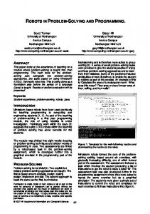
Our test program package was written in C language. The input is compatible with the SMPS format though it relies on special naming conventions that simplify data handling in case of two-stage problems. The structure of our Level Decomposition implementation is depicted in Figure 1. The solver consists of three components: The main module is an implementation of the Inexact Constrained Level Method. An approximation scheme provides recourse and constraint function information in the form of cuts of appropriate accuracy. The CPLEX callable library is used for the solution of the linear and quadratic subproblems arising from decomposition, and for the solution of the recourse problems constructed in the approximation scheme. Our implementation of the Inexact Constrained Level Method includes the bundle reduction technique mentioned in Section 2, which means that inactive cuts are discarded after certain iterations. The dynamically changing bundle is stored in chained lists, where each element represents a single cut (the relevant δ-subgradient and function value are stored). Once a cut is discarded, the appropriate list element is unlinked form the active chain, and linked on the inactive chain. In our implementation of the approximation scheme, the original distribution needs to be discrete. (We approximate a discrete distribution with coarser ones.) We are going to sketch the data structures using the notation of Section 3.1. The cell structure is stored as a binary tree. Leaf elements of the tree represent cells. A cell cut is represented by linking two new leaf elements to the appropriate tree element (which ceases to be a leaf). Given a cell C, the following data are stored in the corresponding leaf element: – the number NC and the total weight pC of those η-realizations that fall into this cell. – coordinates of the barycenter η C . – the gradient of the linear function lC (x), together with the lower approximation LC of F C (ˇ x). The upper ˇ denotes the current iterate of the master problem, in accordance approximation UC of F C (ˇ x). (Here x with the notation of the previous section.) ]

– analogous data for the constraint function: the gradient of the linear function lC (x), together with the ] ] lower approximation LC . The upper approximation UC . The η-realizations are stored in a separate list. Those falling into a given cell are chained to the corresponding leaf element. We also maintain a list of the cell vertices. The vertices of a given cell are chained to the corresponding leaf element. The data structures in our distribution approximation scheme are similar to those proposed by Mayer (1998). He implemented the L-Shaped Method imbedded into a classical approximation scheme. We mention the technical detail that we do not approximate the distribution over cells having NC ¿ 2r˜. For such cells we make exact computation. (The rationale is that for such a cell, η would have more realizations than the original η.) In the present implementation, the recourse problems are solved exactly. (I.e., with high precision. With the notation of the previous section it means working with θ = 0 and hence δ˜ = 0.) The reason for not 20

exploiting inexact solutions is that convergence of the CPLEX optimizer can be controlled through a relative tolerance, while our framework would require using an absolute tolerance. This is a purely technical problem that could be resolved by closer integration of the LP solver. For the solution of the recourse problems we can presently apply either the CPLEX dual simplex optimizer or the CPLEX barrier optimizer. The CPLEX dual simplex optimizer supports warm starts, while the CPLEX barrier optimizer presently does not.

5

Test problems and parameter setting

We tested with variants of the following two problems, taken from the Portable Stochastic Programming Test Set (POSTS) compiled by Derek Holmes. POSTS is available through the Stochastic Programming Community home page: http://stoprog.org. PLTEXPA2 is the linear relaxation of a stochastic capacity expansion problem. Problem sizes are: m = 62, n = 188, r = 104, s = 272. Only the right-hand-side vector d contains random parameters. In the original problem only 7 components are random. STORMG2 is based on a cargo flight scheduling application described by Mulvey and Ruszczy´ nski (1995). Problem sizes are: m = 187, n = 121, r = 526, s = 1259. Only the right-hand-side vector d contains random parameters. In the original problem only 118 components are random. We changed the objective function of the PLTEXPA2 problem. Moreover we changed the distributions of the right-hand-side vectors in both test problems. The distributions we use have nothing in common with the original ones. In our variants, all components of the d vectors are stochastic. In case of the PLTEXPA2 problem, the 104-dimensional ξ ≡ d vector linearly depends on a 6-dimensional random η vector. In case of the STORMG2 problem, there is no linear dependence among the 526 components of the d vector. We created two sets of test problems: PLTEXPA2, standard model. For the problems in this set, the S matrix and the realizations of the η vector were generated in such a manner that the first-stage problems (7) would be feasible. We ˆ ∈ X is selected. (Feasibility of the first-stage problem is sketch the construction: First a point x ˆ a feasible solution.) After this, r˜ points are selected form the translated cone ensured by making x ˆ + { W y | y ≥ 0 }. Let these points be denoted by s1 , . . . , sr˜. For t = 1, . . . r˜, the ray { ust | u ≥ 0 } Tx intersects the translated cone. Let [st , st ] denote the intersection interval. Realizations of η are generated so that Sη falls into the convex hull of the points s1 , s1 , . . . , sr˜, sr˜. (The S matrix is constructed by concatenating the columns s1 , . . . , sr˜.) We created six STOCH files containing 100,000, 200,000, . . . , 600,000 scenarios, respectively. The weight in the objective function was set to w = 2000. This setting assures that Assumption 1 holds, hence we indeed solved a ’traditional’ two-stage recourse problem. The setting w = 2000 was found through trials with different settings. (PLTEXPA2 is a capacity expansion problem, hence the recourse problems have a special combinatorial structure. In our opinion, it is because of this special structure that Assumption 1 holds with such a moderately sized weight.) STORMG2, relaxed model. The realizations of the η vector are samples from the 526-dimensional normal distribution having expectation vector 1 = (1, . . . , 1)T and covariance matrix I. The norm k k¦ = k k1 is used in the objective function with the weight w = 2000. In the constraint G(x) ≤ Γ, we set Γ = 2000. This is an arbitrary choice of parameters. We checked that Γ is large enough to make the relaxed problem (8) feasible. We also checked that Assumption 6 does not hold with the present setting of w. (This is not a ’traditional’ two-stage recourse problem.) 21

We created twenty STOCH files containing 1000, 2000, . . . 20,000 scenarios, respectively. The CORE files of our variants of the test problems, and the STOCH files of our PLTEXPA2 standard model test set are available via the Internet at the address http://www.cs.elte.hu/∼fabian/testproblems. Test runs were made on a personal computer having 1536 MHz CPU clock frequency and 1033 Mb memory. We used Linux operating system. In this project our aim was building a test system in which different options are easily implemented and compared. Efficiency was considered of secondary importance. In case of the PLTEXPA2-variants, we applied the distribution approximation scheme described in Subsection 3.1. The STORMG2-variants were solved without approximation. The starting iterate x1 was always selected by minimizing a randomly generated linear objective function over the feasible polyhedron X. The parameters controlling the underlying convex programming method were set to λ = 0.5, µ = 0.5. In order to set the rest of parameters, we made some preliminary test runs. Let us sum up the results of these preliminary runs: PLTEXPA2-variants. The original PLTEXPA2 problems have the peculiarity that the expected value of perfect information (EVPI) is very small. For PLTEXPA2 16, e.g., the optimal objective value is about −9.47935 and EVPI ∼ 10−6 holds. Though we changed the objective function and the distribution, our PLTEXPA2-variants inherited the above peculiarity. For our problems, the optimal objective value is about 95, 699.908 and EVPI ∼ 0.64 holds. For the solution of these problems we set the starting accuracy to δ1 = 1e6. In order to see the influence of the parameter γ that controls the accuracy prescribed for the oracle, we solved the 600,000-scenario standard-model test problem with different settings. The problem was solved with 8-digit accuracy of the optimal objective value. The data in Table 1 are representative of our results. Larger γ values lead to more iterations, but less cells in the approximation scheme. Solution times show a strong correlation with the number of the LP optimizer calls. These quantities rise towards the endpoints of the examined interval. We decided use γ = 0.15 for the test runs. We found that the standard-model problems are close to having relatively complete recourse. Having started optimization from a point in X \ K, the feasible region X ∩ K was reached in a few master iterations, and infeasibility never occurred in later iterations. STORMG2-variants. The optimal objective values of these problems were between 5, 282, 300 and 5, 282, 600. We found EVPI to be around 4000. For the solution of these problems we set the starting accuracy to δ1 = 1e4. The setting γ = 0 formally expresses that these problems were solved without approximation of the expected recourse function.

6

Test results

Let us sum up details of the tests that were run on the different problem sets: PLTEXPA2, standard model. Problems from this set were solved with four different settings of the optimality tolerance: the solution process was terminated when the accuracy of the optimum reached 5, 6, 7, or 8 digits, respectively. Each problem was solved twice with each setting of the optimality tolerance ; first by using the CPLEX dual simplex solver, and second time, by using the CPLEX barrier solver, for the solution of the recourse problems. When using the dual simplex solver, we exploited the warm-start facility in a scheme described in Section 3.2. When using the barrier solver, we could not exploit the similarity of the recourse problems.

22

Tables 2 - 6 summarize the results of those test runs where warm starts were exploited. In these tables, column headers show the prescribed accuracy in digits. In Tables 3 - 6, row headers show the numbers of the scenarios. Test results of the runs not exploiting warm starts were very much similar to those cited in Tables 2 - 4. (Differences were under 10%.) In solution times, however, we found substantial differences: the barrier solver runs took 50% - 200% more time than the dual simplex solver runs. STORMG2, relaxed model. These problems were solved with 8 digit accuracy of the optimum. The recourse problems were solved by the CPLEX barrier solver. (There is no exploitable similarity in the recourse problems because the random vector is high dimensional and has independent components.) Test results are summed up in Table 7. Table 2 shows that in case of our PLTEXPA2 problem set, the Inexact Constrained Level Method converged at a steady rate: it required 5 or 6 master iterations to achieve an additional exact digit in optimum. However, the effort required for the expected recourse function evaluations grew rapidly with the accuracy prescribed. (The numbers of the cells in the approximation scheme and the numbers of the CPLEX optimizer calls are shown in Tables 3 and 4.) Solution times shown in Table 5 reflect the growing effort of approximation. On the other hand, the effort of the function evaluations did not grow in proportion with the number of the scenarios. Let us consider the solution times in Table 5, and divide each item with the corresponding sample size given in the row header ; these ratios show a decreasing tendency. Algorithmic structure of the Level Decomposition (LD) Method is such that the number of the LD master iterations required to solve a problem is independent of the number of the scenarios. Our test results seem to reinforce this theoretical observation. For both of our test sets, the respective sets of the scenarios can be considered as random samples from the same continuous distribution. In this view, we solved two different continuous problems by Monte Carlo sampling. Sampling of the random parameters is often used in practice, and the estimators of the optimal value and the optimal solution are well investigated. A state-of-art survey can be found in Shapiro (2003). ? ? We mention the following consistency result: Let ON and SN denote the optimal objective value, and the set of the optimal solutions, respectively, of the approximating problem constructed using a sample of size N . Let O? and S ? denote the optimal objective value, and the set of the optimal solutions, respectively, of the true problem. Then ? ON → O? (26) and

? D(SN , S ? ) := sup dist(x, S ? ) x∈SN?

→0

(27)

with probability 1 as N → ∞. (Here dist(x, S ? ) means the distance from x to S ? .) The above consistency result also holds for the relaxed model (8) if the parameter Γ is properly set. (With large enough Γ, the Slater condition is satisfied. Together with the present assumptions, it implies consistency – see Remark 8 in Shapiro (2003).) Our test results are in accordance with (26) and (27). Regarding our first test set, Table 6 shows optimal objective values of our discrete problems for different sample sizes. Regarding our second test set, optimal objective values are shown in the last column of Table 7. The sequence of the optimal objective values seems to converge in both cases, though the convergence is much slower for the relaxed model. In case of the standard model, the sequence of the optimal objective values is noticeably monotonic. This characteristic is explained by the following inequality found by Norkin, Pflug, and Ruszczy´ nski (1998); and Mak, Morton, and Wood (1999): ¡ ? ¢ ? ? IE (ON ) ≤ IE ON (28) +1 ≤ O . This inequality was originally proved for the relatively complete recourse case, but it readily generalizes for the standard (incomplete recourse) model (7). It may not hold for the relaxed model (8), though. 23

The 8-digit optimal solutions of our PLTEXPA2 problems have Euclidean norms of about 540, and they could be covered by a ball having a radius of 0.23. However, the spread is determined by a peculiar flatness of the objective function, rather than by sample sizes: We have solved the same 600,000-scenario problem with 8-digit accuracy several times, and found the spread of the minimizers to be in the magnitude of 1. We mention that if the true problem has a single optimal solution and the ε-optimal set is small for small ε, then minimizers of the sample problems may converge very quickly, and the sequence may even stabilize for relatively small sample sizes. Linderoth, Shapiro, and Wright (2002) present extensive numerical experience regarding this phenomenon, and theoretical explanation was given by Shapiro and Homem-de-Mello (2000). The 8-digit optimal solutions of our STORMG2 problems have Euclidean norms of about 535, and they could be covered by a ball having a radius of 0.68. However, these approximate optimal solutions lie along a straight line in the 121-dimensional space: Projecting them onto a certain hyperplane we got points that could be covered by a ball having a radius of 0.08. This observation is in accordance with that of Linderoth, Shapiro, and Wright who observed that the ε-optimal set of the STORM problem is close to being a short line segment, rather than a large multidimensional basin. (STORM is similar to STORMG2.) Remark 14 The 8-digit accuracy has little practical relevance: In general, probability distributions are coming via statistical estimates which are far less accurate. (In the present cases, the sample sizes allowed only 5-6 accurate digits.) With setting such small stopping tolerances, our aim was only to explore the boundaries of the usability of the method. Let us mention that when we had prescribed an accuracy of no more than 6 digits, we observed quite reasonable solution times even with the present experimental version of the solver.

7

Conclusions and prospects

This paper contains the following new results: – We examine conditions under which the expected recourse function can be extended to the whole space, and identify problem classes where this extension can be done in a computationally efficient way. Network recourse problems constitute such a problem class. Such extension is also necessary in case of two-stage stochastic models using probabilistic constraints, see Prékopa (1995, Chapter 12.10). Hence Proposition 3 and Corollary 9 has application in this field, too. – By using the above extension and by explicitly accounting for infeasibility in the recourse subproblems, we formulate traditional two-stage stochastic programming problems as constrained convex programming problems. This formulation is called standard model in the paper. This approach is practicable only if the expected recourse function can be extended in a computationally efficient way. In general, applicability critically depends on the magnitude of the penalty parameter w. Though Remark 5 justifies a heuristic procedure for setting the penalty parameter. – We propose a new variant of the two-stage recourse model. Called relaxed model in the paper, this can be regarded as a generalization of the well-known integrated chance constrained model of Klein Haneveld (1986). We also give economic interpretations of the relaxed model. One of them substantially differs from traditional two-stage recourse models. It deals with the design and operation of a system that consumes certain resources in whose supply random interruptions may occur. – For the above models, we propose a new solution method, called Level Decomposition in the paper. The method consists of two known components. – The first component is an approximative version of the Constrained Level Method of Lemaréchal, Nemirovskii, and Nesterov (1995). The approximative method was proposed by Fábián (2000). 24

– The second component involves the classic discretization and bounding methods worked out by Kall (1980), Kall and Stoyan (1982), and Birge and Wets (1986). The novelty of Level Decomposition is the way these two components are integrated, and the fact that the master problem is solved by a convex programming method suited for constrained optimization. In a typical implementation of the traditional solution framework, the main module is the distribution approximation scheme, and the submodule is the two-stage stochastic problem solver. To what extent the approximation should be refined between solver calls, is a difficult question, to which Mayer (1998) proposed a heuristic method. In Level Decomposition, the main module is the solver, and the approximating coarse distributions are refined in accordance with the solution process of the master problem. At each step, we have an estimate of how closely the optimum has been approached. At the beginning of the procedure, a rough approximation of the expected recourse function may be used. As the optimum is approached, the accuracy of the function evaluations can gradually be increased through gradual refinement of the approximating distributions. (In a single function evaluation, higher accuracy requires larger effort from the distribution approximation scheme. On the other hand, rough approximations may result in an increased number of iterations. Efficiency requires finding a balance between different efforts. Table 1 contains some experimental results concerning this issue: measures of various computational efforts are presented for different settings of the run-time parameter that controls accuracy prescribed for the approximation scheme.) Using a convex programming method suited for constrained optimization means that feasibility and optimality issues are taken into consideration simultaneously. The bundle-type regularization extends to both feasibility and optimality issues. We avoid feasibility cuts that are constituents of the Benders family of solution methods. The price to be paid is that measuring infeasibility generally requires extra computational effort. Though Remark 13 shows that for certain problem classes, the extra effort is negligible. We report encouraging test results with Level Decomposition. However, its utility can only be assayed by systematic comparisons with benchmark methods. Simplex vs. interior-point methods for the solution of the recourse problems. The cell structure of the distribution approximation offers natural means for batching recourse problems on the basis of similarity. Our test results show that the use of warm starts substantially decreases the time required for the solution of the recourse subproblems. It means that the dual simplex method is a good choice for the recourse problem solver. Efficiency can be enhanced by applying the special dual phase-II method of Maros (2003 A). Interior-point methods are reputed to have difficulties with warm start. However, Gondzio and Grothey (2003) proposed a reoptimization method to overcome these difficulties. They tested their method with an infeasible primal-dual solver, and report a substantial speedup. As a starting point, reoptimization needs a well-centered solution of the former problem. (An optimal solution of the former problem is not suitable, because it is close to the boundary of the feasible region.) This fact luckily coincides with our aim of finding near-optimal solutions. Measuring the utility of interior-point warm starts in Level Decomposition requires further investigation.

7.1

Possible fields of application

Sample Average Approximation. SAA frameworks are an alternative to discretization in case the representation (22) does not hold. In general, batches of sample problems are solved, and some optimality condition is tested by statistical tools. For example, Norkin, Pflug, and Ruszczy´ nski (1998) and Mak, Morton, and Wood (1999) construct confidence intervals for the optimality gap using the inequality (28). Besides estimating optimality gap, Shapiro and Homem-de-Mello (1998) propose another test based on the verification of the Karush-Kuhn-Tucker conditions.

25

Linderoth, Shapiro, and Wright (2002) used these statistical tools in estimating the optimum and in testing for (approximate) optimality. They solved two-stage stochastic programming problems with astronomical numbers of scenarios like 6 × 1081 . They produced good approximate solutions through sampling. (They used a trust-region method on a computational grid for the solution of their sample problems.) If one uses Level Decomposition for the solution of sample problems in SAA frameworks, then the optimality tolerance can be tuned in accordance with sample sizes and with the number of the sample problems. Models with probabilistic constraints. Prékopa (1973) proposed prescribing the feasibility of the recourse problem (1) by a probability ≥ p (with 0 < p < 1, given parameter). In case the random vector has a logconcave distribution, logconcavity of the probabilistic constraint follows from the theory developed by Prékopa (1971). There are effective tools for the estimation of the probabilistic constraint function ; a state-of-art survey can be found in Prékopa (2003). On the other hand, the expected recourse function can be estimated through discretization (or through sampling). The two types of estimation may be used in a common framework. Models with Conditional-Value-at-Risk objectives and constraints. The CVaR risk measure was proposed by Rockafellar and Uryasev (2000). They derived a representation of CVaR that makes it tractable in optimization problems. An overview of CVaR-optimization models and methods can be found in Prékopa (2003) and in Kall and Mayer (2005). Based on the polyhedral representation of K¨ unzi-Bay and Mayer (2006), Fábián (2005, 2006) proposed decomposition frameworks for handling CVaR objectives and constraints in two-stage stochastic models. Approximation of CVaR requires less effort than exact computation. This feature suggests that Level Decomposition may be useful for the solution of such problems.

Acknowledgement The authors would like to thank András Prékopa for suggesting this research and continuous encouragement, and Tamás Terlaky for his constructive remarks concerning the application of interior-point methods. We are grateful to István Maros and to the anonymous Referees for many valuable comments and suggestions that led to substantial improvement of the paper.

References [1] Andersen, E.D. and K.D. Andersen (2000). The MOSEK Interior-Point Optimizer for Linear Programming: An Implementation of the Homogeneous Algorithm. In: High Performance Optimization (H. Frenk, K. Roos, T. Terlaky, and S. Zhang, eds.), Kluwer Academic Publishers, Dordrecht, 197-232. [2] Beale, E.M.L. (1955). On Minimizing a Convex Function subject to Linear Inequalities. Journal of the Royal Statistical Society, Series B 17, 173-184. [3] Benders, J.F. (1962). Partitioning Procedures for Solving Mixed-Variables Programming Problems. Numerische Mathematik 4, 238-252. Re-publised in Computational Management Science 2 (2005), 3-19. [4] Birge, J.R. and F.V. Louveaux (1997). Introduction to Stochastic Programming. Springer-Verlag, New York. [5] Birge, J.R. and R.J.-B. Wets (1986). Designing Approximation Schemes for Stochastic Optimization Problems, in particular for Stochastic Programs with Recourse. In: Stochastic Programming 84 (A. Prékopa and R.J.-B. Wets, eds.), Vol. 1, Mathematical Programming Study 27, 54-102. 26

¨ rck, ˚ [6] Bjo A. (1996). Numerical Methods for Least Squares Problems. Society for Industrial and Applied Mathematics, Philadelphia. [7] Dantzig, G.B. (1955). Linear Programming under Uncertainty. Management Science 1, 197-206. [8] Dantzig, G.B. and A. Madansky (1961). On the Solution of Two-Stage Linear Programs under Uncertainty. In: Proceedings of the Fourth Berkeley Symposium on Mathematical Statistics and Probability Vol. 1, 165-176. University of California Press, Berkeley. [9] Dantzig, G.B. and P. Wolfe (1960). The Decomposition Principle for Linear Programs. Operations Research 8, 101-111. ´ bia ń, C.I. (2000). Bundle-Type Methods for Inexact Data. Central European Journal of Operations [10] Fa Research 8 (special issue, T. Csendes and T. Rapcsák, eds.), 35-55. ´ bia ń, C.I. (2005). Decomposing CVaR Minimization in Two-Stage Stochastic Models. Stochastic [11] Fa Programming E-Print Series 20-2005. ´ bia ń, C.I. (2006). Handling CVaR Objectives and Constraints in Two-Stage Stochastic Models. [12] Fa RUTCOR Research Report 5-2006. [13] Frauendorfer, K. (1988). Solving SLP Recourse Problems with Arbitrary Multivariate Distributions – The Dependent Case. Mathematics of Operations Research 13, 377-394. [14] Frauendorfer, K. and P. Kall (1988). A Solution Method for SLP Recourse Problems with Arbitrary Distributions – The Independent Case. Problems of Control and Information Theory 17, 177-205. [15] Gassmann, H.I. and S.W. Wallace (1996). Solving Linear Programs with Multiple Right-Hand Sides: Pricing and Ordering Schemes. Annals of Operations Research 64, 237-259. [16] Gondzio, J. and A. Grothey (2003). Reoptimization with the Primal-Dual Interior Point Method. SIAM Journal on Optimization 13, 842-864. [17] Kall, P. (1980). Solving Complete Fixed Recourse Problems by Successive Discretization. In Recent Results in Stochastic Programming, Lecture Notes in Economics and Math. Systems 170 (P. Kall and A. Prékopa, eds.), Springer-Verlag, Berlin, 135-138. [18] Kall, P. and J. Mayer (2005). Stochastic Linear Programming: Models, Theory, and Computation. Springer, International Series in Operations Research and Management Science. [19] Kall, P. and D. Stoyan (1982). Solving Stochastic Programming Problems with Recourse including Error Bounds, Mathematische Operationsforschung und Statistik, Series Optimization 13, 431-447. [20] Kall, P. and S.W. Wallace (1994). Stochastic Programming. John Wiley & Sons, Chichester. [21] Kennington, J.L. and R.V. Helgason (1980). Algorithms for Network Programming. John Wiley & Sons, New York. [22] Klafszky, E. and T. Terlaky (1992). On the Ellipsoid Method. Radovi Matematicki 8, 269-280. [23] Klein Haneveld, W.K. (1986). Duality in Stochastic Linear and Dynamic Programming. Lecture Notes in Economics and Math. Systems 274 Springer-Verlag, New York. ¨ nzi-Bay, A. and J. Mayer (2006). Computational Aspects of Minimizing Conditional Value-at[24] Ku Risk. Computational Management Science 3, 3-27.

27

ćhal, C. (1982). Basic Theory in Nondifferentiable Optimization. Research Report No. 181, [25] Lemare Institut National de Recherche en Informatique at en Automatique, Domaine de Voluceau, Rocquencourt, France. ćhal, C., A. Nemirovskii, and Yu. Nesterov (1995). New Variants of Bundle Methods. [26] Lemare Mathematical Programming 69, 111-147. [27] Linderoth, J.T., A. Shapiro, and S.J. Wright (2002). The Empirical Behavior of Sampling Methods for Stochastic Programming. Optimization Technical Report 02-01. Computer Science Department, University of Wisconsin-Madison. [28] Mak, W-K., D. Morton, and R.K. Wood (1999). Monte Carlo Bounding Techniques for Determining Solution Quality in Stochastic Programs. Operations Research Letters 24, 47-56. [29] Maros, I. (2003 A). A Generalized Dual Phase-2 Simplex Algorithm. European Journal of Operational Research 149, 1-16. [30] Maros, I. (2003 B). Computational Techniques of the Simplex Method. Kluwer Academic Publishers, Boston. [31] Mayer, J. (1998). Stochastic Linear Programming Algorithms. Gordon and Breach Science Publishers, Amsterdam. ´ ski (1995). A New Scenario Decomposition Method for Large Scale [32] Mulvey, J.M and A. Ruszczyn Stochastic Optimization. Operations Research 43, 477-490. ´ ski (1998). A Branch and Bound Method for Sto[33] Norkin, V.I., G.Ch. Pflug, and A. Ruszczyn chastic Global Optimization. Mathematical Programming 83, 425-450. ´kopa, A. (1971). Logarithmic Concave Measures with Applications to Stochastic Programming. [34] Pre Acta Scientiarium Mathematicarum (Szeged) 32, 301-316. ´kopa, A. (1973). Contributions to the Theory of Stochastic Programming. Mathematical Pro[35] Pre gramming 4, 202-221. ´kopa, A. (1995). Stochastic Programming. Kluwer Academic Publishers, Dordrecht. [36] Pre ´kopa, A. (2003). Probabilistic Programming. In: Stochastic Programming, Handbooks in Opera[37] Pre tions Research and Management Science 10 (A. Ruszczy´ nski and A. Shapiro, eds.), Elsevier, Amsterdam, 267-351. [38] Rockafellar, R.T. and S. Uryasev (2000). Optimization of Conditional Value-at-Risk. Journal of Risk 2, 21-41. [39] Roos, C., T. Terlaky, and J.-Ph. Vial (1997). Theory and Algorithms for Linear optimization. John Wiley & Sons, Chichester. ´ ski, A. (1986). A Regularized Decomposition Method for Minimizing the Sum of Polyhedral [40] Ruszczyn Functions. Mathematical Programming 35, 309-333. ´ ski, A. (2003). Decomposition Methods. In: Stochastic Programming, Handbooks in Opera[41] Ruszczyn tions Research and Management Science 10 (A. Ruszczy´ nski and A. Shapiro, eds.), Elsevier, Amsterdam, 141-211. ´ ski, A. and A. Shapiro (2003). Stochastic Programming Models. In: Stochastic Program[42] Ruszczyn ming, Handbooks in Operations Research and Management Science 10 (A. Ruszczy´ nski and A. Shapiro, eds.), Elsevier, Amsterdam, 1-64. 28

´ ¸ tanowski (1997). Accelerating the Regularized Decomposition Method ´ ski, A. and A. Swie [43] Ruszczyn for Two-Stage Stochastic Linear Problems. European Journal of Operational Research 101, 328-342. [44] Shapiro, A. (2003). Monte Carlo Sampling Methods. In: Stochastic Programming, Handbooks in Operations Research and Management Science 10 (A. Ruszczy´ nski and A. Shapiro, eds.), Elsevier, Amsterdam, 353-425. [45] Shapiro, A. and T. Homem-de-Mello (1998). A Simulation-Based Approach to Two-Stage Stochastic Programming with Recourse. Mathematical Programming 81, 301-325. [46] Shapiro, A. and T. Homem-de-Mello (2000). On the Rate of Convergence of Monte Carlo Approximations of Stochastic Programs. SIAM Journal on Optimization 11, 70-86. [47] Schrijver, A. (1986). Theory of Linear and Integer Programming. John Wiley & Sons, Chichester. ´ ntai, T. (1988). A Computer Code for the Solution of Probabilistic-Constrained Stochastic Pro[48] Sza gramming Problems. In Numerical Techniques for Stochastic Optimization (Yu. Ermoliev and R.J.-B. Wets, eds.), Springer-Verlag, New York. [49] Van Slyke, R. and R.J.-B. Wets (1969). L-Shaped Linear Programs with Applications to Optimal Control and Stochastic Programming. SIAM Journal on Applied Mathematics 17, 638-663. [50] Wets, R.J.-B. (1974). Stochastic Programs with Fixed Recourse: The Equivalent Deterministic Program. SIAM Review 16, 309-339. [51] Zakeri, G., A.B. Philpott, and D.M. Ryan (2000). Inexact Cuts in Benders Decomposition. SIAM Journal on Optimization 10, 643-657.

29

Inexact Constrained Level Method @

and constraint XXX recourse evaluations XXfunction XXX XXX XX XXX X

Approximation Scheme

@

@

¡ ¡

@

@ linear and quadratic@ @ subproblems

@

¡ @ ¡ @ ¡ CPLEX Callable

¡ ¡ ¡ recourse problems

Library

Figure 1: The structure of our Level Decomposition implementation.

30

γ

iterations

cells

1000 calls

sol.time

0.01

>19

>12,451

>10,892

>2,000

0.03

22

11,984

9,574

1,669

0.06

25

11,637

9,500

1,608

0.09

28

11,203

9,925

1,664

0.12

30

10,652

9,070

1,396

0.15

33

10,352

9,078

1,348

0.18

37

10,284

9,854

1,467

0.21

42

10,213

11,010

1,658

Table 1: Results of preliminary test runs for tuning the run-time parameter γ that controls the accuracy prescribed for the oracle. (The 600,000-scenario PLTEXPA2 standard model was solved with different settings. Stopping tolerance prescribed 8-digit accuracy each time.) Row headers show the different γ settings. Columns contain: numbers of iterations / numbers of cells in the approximation scheme / numbers of CPLEX dual simplex optimizer calls in thousands / solution times in minutes. (The > symbols in the first row indicate that we could not solve the problem with the setting γ = 0.01, due to memory shortage.) Larger γ values lead to more iterations, but less cells in the approximation scheme.

5

6

7

8

17

22

27 - 28

33

Table 2: PLTEXPA2 standard model. Numbers of master iterations required to achieve different numbers of accurate digits in optimum. (Iteration numbers proved virtually independent of the number of the scenarios. In case of 7-digit accuracy, the program made 27 iterations for some scenario numbers, and 28 iterations for others.)

31

5

6

7

8

100,000

110

1,259

1,943

2,205

200,000

30

1,591

3,131

4,080

300,000

27

1,211

3,491

5,096

400,000

26

816

5,033

7,074

500,000

26

523

4,404

7,983

600,000

27

810

6,126

10,352

Table 3: PLTEXPA2 standard model. Numbers of cells in the approximation scheme. (Column headers show the prescribed accuracy in digits. Row headers show the numbers of the scenarios.)

5

6

7

8

100,000

51

680

1,756

2,731

200,000

29

659

2,160

4,347

300,000

29

452

2,296

5,371

400,000

29

290

3,119

6,496

500,000

29

192

2,434

7,168

600,000

28

279

3,381

9,078

Table 4: PLTEXPA2 standard model. Numbers of CPLEX optimizer calls in thousands. (Calls required for the estimation of the expected recourse function and of the infeasibility measure are both counted.)

32

5

6

7

8

100,000

2

64

291

551

200,000

2

32

264

794

300,000

3

19

270

983

400,000

3

11

320

1,049

500,000

3

10

216

1,148

600,000

4

13

264

1,348

Table 5: PLTEXPA2 standard model. Solution times (in minutes) belonging to runs that exploit warm starts. (Recourse problems were solved by the CPLEX dual simplex solver.)

8

100,000

95,699.682

200,000

95,699.817

300,000

95,699.863

400,000

95,699.885

500,000

95,699.899

600,000

95,699.908

Table 6: PLTEXPA2 standard model. Optimal objective values of the sample problems. These data belong to solutions of 8-digit accuracy in optimum. (Row headers show the numbers of the scenarios.)

33

iterations

sol.time

optimum

1,000

23

42

5,282,318.0

2,000

26

93

5,282,339.8

3,000

22

119

5,282,351.4

4,000

26

187

5,282,304.0

5,000

23

207

5,282,329.8

6,000

26

282

5,282,341.7

7,000

22

277

5,282,380.4

8,000

22

316

5,282,380.6

9,000

27

436

5,282,413.7

10,000

30

540

5,282,424.2

11,000

26

515

5,282,427.9

12,000

23

498

5,282,429.6

13,000

23

538

5,282,427.2

14,000

22

553

5,282,443.4

15,000

22

595

5,282,459.7

16,000

22

634

5,282,431.9

17,000

23

706

5,282,444.7

18,000

23

747

5,282,451.2

19,000

25

853

5,282,431.7

20,000

21

755

5,282,424.9

Table 7: STORMG2 relaxed model. Each of these problems was solved with 8-digit accuracy. (Row headers show the numbers of the scenarios. Columns contain: numbers of master iterations / solution times in minutes / optimal objective values.)

34