Application of Stochastic Dynamic Programming in ...

World Applied Sciences Journal 30 (7): 838-843, 2014 ISSN 1818-4952 © IDOSI Publications, 2014 DOI: 10.5829/idosi.wasj.2014.30.07.56

Application of Stochastic Dynamic Programming in Water Allocation, Case Study: Latian Dam 1

1

Hamed Najafi Alamdarlo, 2Majid Ahmadian and 1SadeghKhalilian

Department of Agricultural Economics, TarbiatModares University, Tehran, Iran 2 Faculty of Economics, University of Tehran, Tehran, Iran

Abstract: Optimal allocation and dynamic and stochastic factors in water allocation are important. So In this paper, stochastic dynamic programming (SDP) is used determine the optimum of water allocation to farmers ofVaramin plain and municipal of Tehran city from latian dam during 1991-2012. Objective function is consumer welfare surplus that obtained from the area under the agricultural and municipal water demand functions. To estimate the demand function a panel data approach is used. Given that the operation of the reservoir dam has always been a conflict between the decision makers, the purpose of this paper is determine the optimal allocation of water. Hence, it is assumed the amount of water allocation to farmers it`s not optimal and it`s must be increased. According to results, optimal of water allocation for agriculture and municipal is 220.704 and 383.561 MMC, respectively. Hence, the amount of water allocated to agriculture can be increased. Also, according to demand curve of water, agricultural water supply in drought conditions is necessary. JEL Classification: Q25 D6 C6 C23 Key words: Optimal Water Allocation Stochastic Dynamic Programing INTRODUCTION

Latian Dam

In past years, water scarcity has become threat in most arid and semiarid regions around the world, including reservoir [6] and much research has been conducted using reservoir optimization models to identify optimal operating strategies [7]. But, in water resources management, uncertainties could intensify the conflictladen issue of water allocation among competing municipal, industrial and agricultural interests. Consequently, to address the uncertain parameters Stochastic Dynamic Programming (SDP) was applied to reservoirs management [8-12]. In stochastic programming uncertain parameters are treated as random variables with a known probability density function (PDF). Hence, the consequences of the decisions taken at present re not known until the unknown data is realized.Application of value iteration approach to obtain the value function that solves the Bellman equation, which is adopted mainly as an acceleration method [13-15]. The objective of this paper is to analyze the optimal water allocation of Latian dam reservoir between municipal and agricultural users. For this purpose, Stochastic Dynamic Programming (SDP) has been applied. The basic part of this study are presented as follows.

Reservoir system managements are designed for determining water release by considering the interests of the reservoir stakeholders, inflows, impounded water volume, release capacity, water demands and downstream constraints [1]. This multiple activities and objectivescomplicated supply-demand conflicts [2]. While the demand of water reaches a limit of what the natural system can provide, water shortage will become a major obstacle to social and economic development for one region [3]. More urban regions where demands outstrip water resources availabilities have suffered from chronic severe shortages, particularly when faced with the rapid population increase and speedy economic development. This competitiveness can strengthen the agricultural water shortage and serious problems (e.g. agricultural sustainability concerned) can thus arise from poorly planned water-management systems when merely limited water resources are available for multiple competing users [4]. For years, controversial water-allocation issues among municipal, industrial and agriculturalusers have been intensifled [5].

Corresponding Author: Hamed Najafi Alamdarlo, Department of Agricultural Economics, TarbiatModares University, Tehran, Iran

838

World Appl. Sci. J., 30 (7): 838-843, 2014

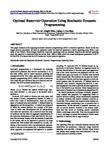
Fig. 1: Latian Dam and Water Allocation between Municipal and Agriculture xt+1 = g(xt,wt) , wt

In Section 2, data collection and case study has been described. In section 3, the methodology of the paper is presented along with the value iteration approach and SDP model. The empirical analysis and the model application results in the study area are analyzed in Section 4. Finally, a conclusion is given in Section 5.

0

(1)

The functional form that chosen for the polynomial approximation to the infinite-horizon is a Chebychev Polynomial, which belongs to a family of orthogonal polynomials described by Judd [13] and implemented by Provencher and Bishop [15]. The approximation takes the form:

Case Study and Data: The Latian Dam is located on Jajrood River in the northeast of Tehran the capital of Iran (Figure 1). It is one of the most important municipal and agricultural water supply reservoirs in Tehran city and Varamin Plain. Also, TheLatian Reservoir is a moderately eutrophic, with an area of 3.3 km2 and a drainage area of 670 km2. This reservoir water to provide 6000 hectareof arable Varamin plain and 30% of Tehran drinkable water. Data is collected from Ministry of Agriculture, Water Resources Management Company of Iran and 240 questionnaires in 2011-2012.

V ( xt ) =

∑

i i

( M ( x ))

(2)

Where i is the coefficient of the ith polynomial term i (M(x) which is defined over the interval given by the mapping x = M ( x ) , that is [-1,1] in thecase of the Chebychev polynomial. The expressions of the Chebychev polynomial aresinusoidal in nature and are given (for the nth term) by the relationship x = Cos n. Cos −1 ( x ) .

(

MATERIALS AND METHODS

)

Stochastic Dynamic Programming Model: Uncertainty in water resources management could be due to the dynamics of the ecosystem or exogenously caused by weather, prices, orinstitutions. SDP approach is the dominant method to solving the discrete time stochastic dynamic equations of motion.This method has been concentrated in optimalnormative intertemporal water allocation. Equation 3, represented a resource network based on a singlestate representation in a network system. The dynamics of the system are givenby:

The Value Iteration Approach: In this approach, a numerical approximation to the infinite horizon valuefunction has used that maximizes the value of the problem resulting from decisions carried out inthe future. For a generic objective function f(xt,wt) and an equation of motion for the state variable xt+1 = g(xt,wt) the Bellman equation is: t   1  MaxV = ( x t )  f ( xt , wt ) +   V ( xt +1 )  1+ r    Subject to

839

World Appl. Sci. J., 30 (7): 838-843, 2014

(3)

∆X t = et′ − Wt

in order to maximize the accumulated value over time. At each year, the level of a state variable is a function of the state variable level at the previous year, the control and the realized stochastic variables, (6). The problem is limited by feasibility constraints. At every year, the current net surplus depends on the water releases. Consequently the objective function is the expectation of the current net surplus. Instead of the traditional methods of optimizing the value function for discrete points in the probability, control and state spaces, two approximations have made, the value function and information accumulation by the decision-maker. We approximate the expected value function by supposing that it is a continuous function in state space. In addition, it is assumed that the decisionmaker at any year regards the stochastic control problem as a closed loop problem based on the recent information. This information is obtained with respect to the amount of water release, to be updated each time by stochastic condition. Implicitly, this approximation suppose that the ability of the decision-maker to observe the updated level of the state variable in the future does not alter the current optimal control given the current state of the system.

The change reservoir stock must balance the stochastic change e1t and resource use wt. The index t in equation (3) denotes time period. The final demand for resourceservices is satisfied by resource flows from Xt, namely wt. We define the following timing of information and controls. First, the decision-maker observes the realization of the exogenous stochastic stock change variable e1′ and hence Xt. Second, the decision-maker chooses the control wt, the level of resourceextraction or harvest. P(W) is the intermediate value of flow resources that defined by the inverse demand FunctionThis function is P = g+k.W, where P is water price, W is water consumption for agriculture and municipal sector and g and k are the intercept and the price coefflcient. The net surplus, CS(w) derived from water consumption is denotedby: (4)

∫

CS ( w ) = P ( w ) , dw

The Surplus of Water Consumption Is a Concave Increasing Function: The optimal decision for all years is same, if the time horizon is infinite. The stochastic dynamic recursive equation that defines the optimal water management is: r

Municipal Demand: Estimates of municipal water demand function are based on water price, per capita income and climate parameters and water demand in this sector is sensitive to price, but is inelastic[16], [17]. Municipal water demand is derived using Stone-Geary function and it is estimated using the random effects model The price elasticity of municipal water demand function has obtained from this literature; [18],[19],[20], [21]. A simple linear form is fitted to the resulting data yielding.

 1   MaxVt (= X t , et ) CSt ( wt ) +  Vt +1 ( X t +1, et ) .dF     1 + r   (5) Sujbect to,

∫

∆X t = et − wt

(6)

X ≤ X t +1 ≤ X

(7)

wt

(8)

0

Agricultural Demand: Agricultural water demand is calculated according to irrigation requirements based on crop areas and climate. Irrigation requirements of crops were estimated using the Penman-FAO-Monteith approach based on climate and crop culture in Varamin plain [22]. To estimate the agriculture water demand function in Varamin plain, a statistical survey has been conducted on a sample of 240 farmers with 8 crops. The water demand function is: Wit = 0 + itXit, that W is water consumption, is parameter and X denote the vector of independent variable (price of water per cubic (10 Rials), Net Revenue (Million Rilas per Hectare) and Climateparameters (temperature and Precipitation)). This equation was estimated with Evewis and Panel Data Approach.

In this equation, X denote a vector of state variables, w a vector of control variables and e a vector of random events that influence the state variables, the objective function or both. r isinterest rate. The distribution of the stochastic vector is known, a priori. The objective function (5) is maximizedto obtain the optimal set of controls w1* ,..., wT* subject to (6), (7) and (8). The objective

{

}

function defined as the discounted sum of net consumer surplus for agriculture and municipal users. The objective of the decision maker is to obtain an optimal water release 840

World Appl. Sci. J., 30 (7): 838-843, 2014

RESULT

Table 1: Water demand priceElasticity Agriculture Municipal

Agriculture and Municipal Water Demand Function: The results of agriculture and municipal water demand function are presented inin the Table 1. Price is inelasticity in both function, but elasticity is agriculture is less than municipal. Using these parameters, intercept and slope can be achieved.So, the consumer surplus of water demandachieved for farmers and households (equation 4).

Intercept

Slope

348.82 330.35

-1.58 -0.7

Resource: Research Finding Table 2: Chebychev polynomial coefficients in Agriculture and municipal model 1 Agriculture 132471 Municipal 320103

2

3

4

5

6

7

21671 -8244 1493.8 -575.1 262.7 117.2 26401.8 -4659.7 1110 -192.2 -62.9 79.5

Resource: Research Finding

Application of Sdp in Latian Reservoir: The Latian Dam Reservoir can be modeled as a single aggregated reservoir and release to the Varamin Plain irrigators and Tehran population water. Accordingly, X is the stock of water in Latian reservoirs, et are the stochastic levels of inflow to the reservoir, w are the water releases from the reservoir that produce water supply for irrigation and drinking. It’s supposed that yearly inflows are i.i.d distributed with a log-normal distribution et i, i.dLN , 2 .

(

Elasticity -0.216 -0.326

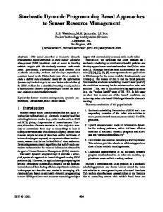
To evaluate the quality of fit of SDP model, it’s simulated the optimal predictedreleases and storage for Latian reservoirs over the historic time period, using the actualrealized inflows to set the initial conditions for each year’s optimization. Figure 1-Ato 1-D presents the SDP policy simulations versus the observed ones for water release (the control) and storage (the state). The information used by decision-maker, namely the current reservoir storage level, the current runoff and the probability distribution of stochastic inflows. The optimization at each time,the marginal value of current releases must be equal to the expected value of water stored and carried over for use in next years. The comparison between the simulated flfland actual amounts allocated water to agriculture and drinking consumers, showed in figure 1-A and 1-B. As this chart shows, the dynamic stochastic programming model is well able to simulate the amount of allocated water and there is a little difference between the actual and simulated. Therefore, the output from the models is reliable. In Figure 1-C and 1-D, the total amount of reservoir water in the two models are compared.Values flsimulated is more suitable in agricultural model. The amount of water allocated to farmers has more random change, but the amount of water allocated to farmers have not changed much. Because in the stochastic conditions, the amount of water allocated to agriculture is associated with greater changes. The value of every unit of water in every year for agriculture and municipal presented in Figure 2-A and 2B.This value obtained by dividing the current value to the amount of water allocated. This function is more elasticity for Municipal users to Agricultural users. Average value of municipal and agricultural water are 237.77and 413.74 (10 Rials), respectively. Given that the price elasticity of water demand is less for farmers, thus, every unit of water is more valuable to theme and are willing to pay more price for water consumption.Therefore, in drought years, the agricultural water must be provided.

)

The maximum and minimum storage capacity in the Latian dam each year is 685 and 209 MCM, respectively. Data on actualinflows, releases and storage are available for 1991 to 2012. A log-normal distributionwas fitted to the observations and used to generate a set of 5 and 4 discrete probabilities forthe associated inflow quantities for municipal and agriculture, respectively. The decisionmaker is assumed to maximize the sum ofthe expected net present value of the water releases over this time period. The objective function maximize subject to the equation of motion for the reservoir stock and thefeasibility constraints. The problem is solved using NLP procedure with GAMS package. A seven degree Chebychev polynomial approximation of the value function is obtained. This polynomial coefficients are iteratively computed using the Chebychev regression algorithm. Table 2 shows the Chebychev polynomial coefficients. In Table 3 are shown the results of maximizing the objective function. The NPV is higher for urban consumers to Agricultural consumers. The optimal amount of water allocated to urban is more than farmers, because they won more prosperity and are willing to pay a higher price for water. The optimal amount of water allocated to farmers and urbanites are higher than longterm averages (72.5 and 121.6 MCM, respectively). Hence, the two groups are demanding more water for consumption. 841

World Appl. Sci. J., 30 (7): 838-843, 2014 Table 3: Optimal water allocation and value of objective function Agriculture

Municipal

1

2

3

4

Stochastic water inflow (MCM) NPVW (10 Rials) Probability Value of Objective Function (10 Rials) Annual Water Allocation (MCM)

16.41 147120.5 0.22 134592.4 220.704

74.14

204.23

315.41

5

0.26 139775.77

0.32 146658.17

0.22 147196.8

Stochastic water inflow (MCM) NPVW (10 Rials) Probability Value of Objective Function (10 Rials) Annual Water Allocation (MCM)

140.27 342383 0.045 323411.160 383.561

231.38

276.78

286.72

295.84

0.27 331563.507

0.36 335144.736

0.27 335883.945

0.045 336547.7

Resource: Research Finding

Fig. 1-A: Compare between actual and simulation of agricultural water allocation

Fig. 1-C: Compare between actual and simulation of Total water allocation in Agri-Model

Fig. 1-B: Compare between actual and simulation of Municipal water allocation

Fig. 1-D: Compare between actual and simulation of Total water allocation in Muni-Model

CONCLUSION

municipal is 220.704 and 383.561 MMC, respectively. Hence, the amount of water allocated to agriculture and municipal can be increased. Also, according to demand curve of water, agricultural water supply in drought conditions is necessary.

In water resources management, uncertainties could intensify the conflict-laden issue of water allocation among competing municipal, industrial and agricultural interests. Hence, in this study, the optimal allocation between farmers and municipal has been investigated by using stochastic dynamic programming in latian Dam at 1992-2012. SDP approach is the dominant method to solving the discrete time stochastic dynamic equations of motion. This method has been concentrated in optimal normative inter temporal water allocation. The result show that optimal of water allocation for agriculture and

REFERENCES 1. Khan, N.M. and T. Tingsanchali, 2009. Optimization and simulation of reservoir operation with sediment evacuation: a case study of the Tarbela Dam, Pakistan. Hydrological Processes, 23: 730-747. 842

World Appl. Sci. J., 30 (7): 838-843, 2014

2. ICOLD, 2007. Dams and the world’s water. International Commission on Large Dams, pp: 64. 3. Bronstert, A., A. Jaeger, A. Ciintner, M. Hauschild, P. Döll and M. Krol, 2000. Integrated modeling of water availability and water use in the semi-arid northeast of Brazil. Physics and Chemistry of the Earth (B) 25(3): 227-232. 4. Le Ngo, L., H. Madsen and D. Rosbjerg, 2007. Simulation and optimization modelling approach for operation of the Hoabinh reservoir, Vietnam. Journal of Hydrology, 336: 269-281. 5. Maqsood, I., G.H. Huang and J.S. Yeomans, 2005. An interval-parameter fuzzy two stage stochastic program for water resources management under uncertainty. European Journal of Operational Research, 167: 208-225. 6. World Water Assessment Program, 2006. Water, a Shared Responsibility. The United Nations World Water Development Report 2. UNESCO-Berghahn Books, New York. 7. Chang, Y.T., L.C. Chang and F.J. Chang, 2005. Intelligent control for modeling of real-time reservoir operation, part ii: arti?cial neural network with operating rule curves. Hydrological Processes, 19: 1431-1444. 8. Yeh, W., 1985. Reservoir management and operations models: a state-of-the-art review. Water Resources Research, 21(12): 1797-1818. 9. Faber, B.A. and J.R. Stedinger, 2001. Reservoir optimization using sampling SDP with ensemble stream ?ow prediction forecasts. Journal of Hydrology, 249(1-4): 113-133. 10. Howitt, H., S. Msangi, A. Reynaud and K.C. Knapp, 2005. Calibrated Stochastic Dynamic Models For Resource Management. American. Journal of Agricultural Economic. 87(4): 969-983 11. Li, Y.P., G.H. Huang, G.Q. Wang and Y.F. Huang, 2009. FSWM: A hybrid fuzzy-stochastic watermanagement model for agricultural sustainability under uncertainty. Agricultural Water Management 96: 1807-1818. 12. Dai, Z.Y. and Y.P. Li, 2013. A multistage irrigation water allocation model for agricultural land-use planning under uncertainty. Agricultural Water Management, 129: 69- 79.

13. Judd, K.L., 1998. Numerical Methods in Economics. M.I.T Press. Cambridge. 14. Bertsekas, D.P. and J.N. Tsitsiklis, 1996. Neuro-dynamic programming. Belmont, Massachusetts. Athena Scienti?c. 15. Provencher, B. and R.C. Bishop, 1997. An Estimable Dynamic Model of recreation Behavior with an Application to Great Lakes Angling. Journal of Environmental Economics and Management, 33(2): 107-127. 16. Xayavong, V., M. Burton and B. White, 2008. Estimating urban residential water-demand with increasing block prices: The case of Perth, Western Australia.” Working Paper 0704, the University of Western Australia. 17. Hoffmann, M., A.C. Worthington and H. Higgs, 2006. “Urban water demand with fixed volumetric charging in a large municipality: The case of Brisbane, Australia.” Australian J. of Agricultural and Recourse Economics, 50(3): 347-359. 18. Pajoyan, J. and S.H. Hoseini, 2001. Estimate of Household Water Demand, Case Study: Tehran City. Journal of Iranian Economic Reserches, 16: 47-67. (In Persian, with English abstract). 19. Sajjadifar, S.H., 2005. Economic evaluation of residential water demand (A Case Study of Arak).” M.Sc. Thesis, Institute of Higher Education and Research in Management and Planning. (In Persian, with English abstract). 20. Sabouhi, M. and M. Nobakht, 2009. Estimating water demand function of Pardis. J. of Water and Wastewater, 70: 69-74. (In Persian, with English abstract). 21. Mousavi, S.N., H. Mohammadi and F. Boostani, 2010. Estimation of water demand function for urban households: A case study of Marvedasht. J. Water and Wastewater, 74, 90-94. (In Persian, with English abstract). 22. Jensen, M.E., R.D. Burman and R.G. Allen 1990. Evapotranspiration and irrigation water requirements. ASCE Manual and Rep. on Engrg. Pract. 70. ASCE, New York.

843