An Approach to Modelling and Verification of Component Based Systems G. Gössler(1) , S. Graf(2) , M. Majster-Cederbaum(3) , M. Martens(3) , J. Sifakis(2) (1)
(2) (3) INRIA Rhône-Alpes VERIMAG University of Mannheim Montbonnot, France Grenoble, France Mannheim, Germany
[email protected] {graf,sifakis}@imag.fr
[email protected]
Abstract. We build on a framework for modelling and investigating componentbased systems that strictly separates the description of behavior of components from the way they interact. We discuss various properties of system behavior as liveness, local progress, local and global deadlock, and robustness. We present a criterion that ensures liveness and can be tested in polynomial time.
1
Introduction
Component-based design techniques are an important paradigm for mastering design complexity and enhancing reusability. In the abstract data type view or object-oriented approach subsystems interact by invoking operations or methods of other subsystems in their code and hence rely on the availability and understanding of the functionality of the invoked operations. In contrast to this, components are designed independent from their context of use. Components may be glued together via some kind of gluing mechanism. This view has lead some authors, e.g. [3,8,21,9] to consider a component as a black box and to concentrate on the combination of components using a syntactic interface description of the components. Nevertheless, for these techniques to be useful, it is essential that they guarantee more than syntax-based interface compatibilities. No matter if a certain functionality has to be established or certain temporal properties must be ensured, knowledge about the components has to be provided. Methods based on the assume-guarantee paradigm [23] or similarly on the more recent interface automata [10] are useful e.g. for the verification of safety properties provided that they can be easily decomposed into a conjunction of component properties. Other approaches rely on some process algebra as CSP or π − calculus [22,17,1] and consider congruences and reductions to discuss properties of component systems. We build here on a framework for component-based modelling, called interaction systems, that was proposed in [14,15,13,24], which clearly separates interaction from (local) behavior of components. In [15] a notion of global deadlock-freedom, called interaction safety there, was introduced and investigated for interaction systems. Here, we explain how the framework can be used to discuss properties of systems including liveness, progress of subsystems, robustness and fairness. In most cases direct testing of the properties relies on an exploration of the global state space and hence cannot be performed efficiently. E.g. we have shown that deciding local and global deadlock-freedom as well as deciding liveness is NP-hard for component-based systems [20,19]. Alternatively one may establish conditions that entail a desired property and that can be tested more efficiently. In [13] a first condition was given that entails global deadlock-freedom of interaction systems. In [18] we established a condition that entails local deadlock-freedom of interaction systems and that can be tested in polynomial time.
Here we present a condition that can be tested in polynomial time and guarantees liveness of a component, of a set of components or of an interaction in an interaction system. We present here a simple version of the framework without variables. In section 1 we introduce the framework and model a version of the dining philosophers as an interaction system. In section 2 we consider properties of interaction systems and illustrate them by examples. In section 3 we present and analyze a condition for liveness that can be tested in polynomial time. Section 4 discusses related and future work.
2
Components, Connectors and Interaction Systems
We build on a framework of [13,15] where components i ∈ K together with their port sets Ai are the basic building blocks. Each component offers an interface which is here given as a set of ports. Each component i has a local behavior that is here given by a local transition system Ti . The local transition system regulates the way in which ports are available for cooperation with the environment. Components can be glued together. The gluing is achieved by a set of connectors. A connector is a set of ports where no two ports belong to the same component. An interaction is a subset of a connector. Certain interactions may be declared as complete interactions. If an interaction is declared complete, it can be performed independently of the environment. If an interaction is complete, so should be all its supersets. Given the above ingredients we define the notion of an interaction system with a global behavior that is obtained from the local transition systems by taking the connectors into account, more formally: Definition 1 Let K be a set of components, Ai , i ∈ K, a port set that is disjoint from the port set of every S other component. Ports ai , bi ... ∈ Ai are also referred to as actions. The union A = Ai of all port sets is the port set of K. A finite nonempty subset c of i∈K
A is called a connector, if it contains at most one port of each component i ∈ K. A connector set is a set C of connectors where: a) every port occurs in at least one connector of C, b) no connector contains any other connector. For connector set C we denote by I(C) all non empty subsets (called interactions) of the connectors in C, i.e. I(C) = {β 6= ∅ | ∃c ∈ C β ⊆ c}. We abbreviate I(C) to IC for ease of notation. The elements c ∈ C are maximal in IC with respect to set inclusion and are hence called maximal interactions. A set U ⊆ IC of interactions is said to be closed w.r.t. IC, if whenever u ∈ U and u ⊂ v ∈ IC then v ∈ U . Let Comp be a closed set of interactions. It represents the complete interactions. Let for each component i ∈ K a transition system Ti = (Qi , Ai , →i ) be given, where a →i ⊆ Qi × Ai × Qi . We write qi →ii qi0 for (qi , ai , qi0 ) ∈→i . We suppose that Qi ∩ Qj = ∅ for i 6= j. In the induced interaction system, the components cooperate via interactions in IC. For the notion of a run and the properties studied in this paper only interactions in C ∪ Comp will be relevant but for composition of systems as in [11] we need all interactions hence they are admitted (as labels) in the following definition. The induced interaction system is given by Sys = (K, C, Comp, T ), where the global behavior T = (Q, IC, →) is obtained from the behaviors of individual components, given by transition the systems Ti , in a straightforward manner: 2
Q – Q = i∈K Qi , the Cartesian product of the Qi , which we consider to be order independent. We denote states by tuples (q1 , ..., qj , ...) and call them global states. – the relation →⊆ Q × IC × Q, defined by α ∀α ∈ IC ∀q, q 0 ∈ Q q = (q1 , ..., qj , ...) → q 0 = (q10 , ..., qj0 , ...) iff i(α)
∀i ∈ K (qi →i qi0 if i participates in α and qi0 = qi otherwise). where for component i and interaction α, we put i(α) = Ai ∩α and say that component i participates in α, if i(α) 6= ∅. The set of states in which ai ∈ Ai is enabled is denoted a by en(ai ) = {qi ∈ Qi | qi →i qi0 for some qi0 } The following example shows how the model of interaction systems can be used to model a solution for the dining philosopher problem. Example 1 We assume that there are n philosophers as well as n forks. The alphabet of philosopheri i = 0, ..., n − 1 is (i+1)mod n
{activatei , enteri , getii , geti
(i+1)mod n
, eati , putii , puti
, leavei }.
The alphabet of f orki is {geti , puti }. To achieve deadlock-freedom we introduce a control component. The alphabet of the control component control1 is {enter, leave}. We introduce the following connectors eat = {eat0 , eat1 , ...eatn−1 }, where any nonempty subset is declared to be complete. act = {activate0 , activate1 , ...activaten−1 }, and for i = 0, ..., n − 1 {enter, enteri }, {leave, leavei }, (i+1)mod n {getii , geti }, {geti , get(i+1)mod n }, (i+1)mod n i {puti , puti }, {puti , put(i+1)mod n }. The transition systems are given by f orki :
control1 :
fi,0
puti
enter c1,0
geti
enter
enter c1,n−1
leave
leave
c1,1 leave
fi,1 philosopheri : leavei
pi,0
activatei
pi,1
pi,7
enteri pi,2
(i+1)mod n
getii
puti
pi,6
pi,3
putii pi,5
eati
pi,4
(i+1)mod n
geti
E.g. act is the only interaction in C ∪ Comp that may take place in the global state q0 = (p1,0 , ..., f1,0 , ..., c1,0 ). Then, {enter, enteri } can take place for a philosopher i. 3
3
Properties of Interaction Systems
We consider in the following several essential properties of component based systems and show how they can be clearly defined in our setting. In what follows, we consider an interaction system Sys = (K, C, Comp, T ) where T = (Q, IC, →) is constructed from given transition systems Ti , i ∈ K, as described in Definition 1. Let P be a predicate on the global state space. We assume here that P is an α inductive invariant, i.e. ∀q, q 0 ∈ Q ∀α ∈ C ∪ Comp (P (q) ∧ q → q 0 ⇒ P (q 0 )). As an example we consider the predicate Preach(q0 ) describing all global states that are reachable (via interactions in C ∪ Comp) from some designated starting state q0 . The first property under consideration is P -deadlock-freedom which is a generalization of the concept of deadlock-freedom of [13,15]. An interaction system is considered to be P -deadlock-free if in every global state that satisfies P it may perform a maximal or complete interaction. This definition is justified by the fact that both for complete and maximal interactions there is no need to wait for other components to participate. Deadlock-freedom is an important property of a system. But it does not provide any information about local deadlocks in which some set ∅ = 6 K 0 ⊆ K of components might be involved and hence we consider this situation as well. Definition 2 Let Sys be an interaction system. Sys is called P -deadlock-free if for every state α q ∈ Q satisfying P there is a transition q → q 0 with α ∈ C ∪ Comp. Let K 0 ⊆ K, K 0 6= ∅. K 0 is involved in a local P -deadlock in state q satisfying P , if for any i ∈ K 0 and for any ai ∈ Ai if qi ∈ en(ai ) then for any α ∈ C ∪ Comp with ai ∈ α there is some j ∈ K 0 and some aj ∈ Aj ∩ α such that qj ∈ / en(aj ). Sys is called locally P -deadlock-free if in any P -state q there is no ∅ = 6 K 0 ⊆ K that is involved in a local P -deadlock in q. For P = true we speak of (local) deadlock-freedom. Remark 1 If Sys is locally P -deadlock-free then it is P -deadlock-free. The converse does not hold. In addition to deadlock-properties it is interesting to consider the property of P progress of K 0 , i.e. the property that at any point of any P -run of the system, there is an option to proceed in such a way that some component of K 0 will eventually participate in some interaction. A subset K 0 of components is said to be P -live if K 0 participates infinitely often in every P -run. Please note that we admit only transitions labelled by elements in C ∪ Comp for the definition of a P -run. Definition 3 Let Sys be a P -deadlock-free interaction system. A P -run of Sys is an infinite sequence α α σ = q0 →0 q1 →1 q2 . . . where ql ∈ Q and P (ql ) = true and αl ∈ C ∪ Comp for any l. αn−1 α α For n ∈ N, σn denotes the prefix q0 →0 q1 →1 q2 . . . → qn . Let ∅ = 6 K 0 ⊆ K. K 0 may P -progress in Sys, if for any P -run σ of Sys and for any n ∈ N there exists σ 0 such that σn σ 0 is a P -run of Sys and some i ∈ K 0 participates in some interaction α of σ 0 . K 0 ⊆ K is P -live in Sys, if every P -run of Sys encompasses an infinite number of transitions where some i ∈ K 0 participates, i.e. for every P -run σ and for all n ∈ N there is an m with m ≥ n and there is i ∈ K 0 with i(αm ) 6= ∅. An interaction α ∈ IC 4
β
is P -live, if every P -run encompasses an infinite number of transitions q → q 0 with α ⊆ β. Sys is called P -fair if every component i ∈ K is P -live in Sys. If P = true, we speak of liveness, similarly we speak of runs, fairness etc. Also we identify a singleton set with its element. Remark 2 If Sys is P -deadlock-free and at least one state satisfies P then P -runs exist as P is an inductive invariant. Lemma 1 Let Sys be P -deadlock-free, ∅ = 6 K 0 ⊆ K. If K 0 may P -progress then K 0 is not involved in a local P -deadlock in any P -state. If Sys is locally P - deadlock-free this does not imply that every component may P -progress. Proof: see Appendix If we consider a setting where a component may involve a technical device, as e.g. in an embedded system, that may break down, we might be interested to know how the properties behave on the failure of that component. As an example we treat here deadlock-freedom and progress. Definition 4 Let Sys be a deadlock-free interaction system. In Sys, deadlock-freedom is called robust with respect to failure of port ai ∈ Ai , if in every state q ∈ Q there is a α transition q → q 0 with α ∈ C ∪ Comp and ai 6∈ α. In Sys deadlock-freedom is called robust with respect to failure of component i, if in every state q ∈ Q there is a α transition q → q 0 with α ∈ C ∪ Comp and i(α) = ∅. Let in Sys deadlock-freedom be robust with respect to failure of port ai ∈ Ai . Suppose that j ∈ K, i 6= j, may progress in Sys. The progress property of {j} is robust with respect to failure of port ai ∈ Ai , if for any run σ of Sys and for any n ∈ N there exists σ 0 such that σn σ 0 is a run of Sys and such that there is some interaction α of σ 0 with j(α) 6= ∅ and no interaction of σn σ 0 contains ai . Remark 3 The philosopher system in Example 1 is Preach(q0 ) -deadlock-free where q0 = (p1,0 , ..., f1,0 , ..., c1,0 ). This is due to the control component that admits at most n − 1 philosophers to the table. By a pigeon hole argument at least one philosopher can get both forks and continue. When he leaves, another philosopher may be admitted to the table. As we will see in section 1 each philosopher is Preach(q0 ) -live in the system and will eat at some time. Hence the system is Preach(q0 ) -fair. In the following we show how we can model a system of n identical tasks that have to be scheduled as they all need the same resource in mutual exclusion. Here no explicit representation of a scheduler or a controller is used. For this example we introduce a rule of maximal progress. The maximal progress rule restricts the transition relation α for Sys to maximal transitions, i.e. to those transitions such that q → q 0 , implies that β there is no β, q 00 with α ( β and q → q 00 . Example 2 We consider a set of tasks Ti (i ∈ K = {1, ..., n}) that compete for some resource in mutual exclusion. The basic behavior of each task is given in Figure 1 and needs not to be further explained. Let the set of ports of each component i be: Ai = {activatei , starti , resumei , preempti , f inishi }. 5
inaci
activatei
f inishi
waiti
starti preempti suspi
execi resumei
Fig. 1. Basic behavior of each task Ti
We want to guarantee mutual exclusion with respect to the exec state, i.e. no two tasks should be in this state at the same time, in the sense that this is an inductive invariant. Mutual exclusion, in this sense, can be achieved using the rule of maximal progress and by the following connectors: for i, j ∈ K, i 6= j, conni1 = {activatei }, connij 2 = {preempti , startj }, connij = {resume , f inish }. {start } and {f inish } are defined i j j j 3 to be complete. Let Systasks be the system defined this way. Observation 1: On every run starting in a state where no two components are in their exec state Systasks guarantees mutual exclusion with respect to the exec state due to the rule of maximal progress. For detailed explanations see appendix. Observation 2: Let P = (∃i qi 6= suspi ). P is an inductive invariant and Systasks is P -deadlock-free and each component i may P -progress. The property of P -deadlockfreedom is robust with respect to failure of the operation resumei . Observation 3: Let P 0 = true then Systasks is not P 0 -deadlock-free as in the state q = (susp1 , ..., suspn ) no interaction in C ∪ Comp is available. We may modify the system by introducing a new action reseti for each i and by enriching the transition system Ti with an edge labelled reseti from the state suspi to inaci . In addition we introduce a connector conng = {reset1 , ..., resetn }. The resulting system Sys0tasks is P 0 deadlock-free. P 0 -Deadlock-freedom is not robust with respect to failure of port reseti and hence not robust with respect to failure of component i, i ∈ K. Alternatively we might consider the state q0 = (inac1 , ..., inacn ). The state q = (susp1 , ..., suspn ) is not reachable from q0 and Systasks is Preach(q0 ) -deadlock-free. Observation 4: When a finite interaction system is P -deadlock-free for some in inductive invariant P , then it is also P -deadlock-free when we apply the rule of maximal progress. Observation 5: In Sys0tasks every component may P 0 -progress under the rule of maximal progress. For detailed explanation see appendix. 6
4
Testing Liveness of Components in Interaction Systems
In the previous examples we have verified some properties of the systems directly. As the properties are conditions on the global state space, they cannot be established directly in an efficient way in general. E.g. we have shown that deciding local and global deadlock-freedom as well as deciding liveness is NP-hard for component-based systems [20,19]. However, one may define (stronger) conditions that are easier to test and entail the desired properties. In [15], a condition for deadlock-freedom of an interaction system (called interaction safety there) is presented that uses a directed graph. The absence of certain cycles in some finite subgraph ensures deadlock-freedom of the system. This criterion can be extended to P -deadlock-freedom, it can be modified to ensure local progress as well as robustness of P -deadlock-freedom with respect to the failure of a port or a whole component, and it can be extended to apply to a broader class of systems including various solutions for the dining philosophers. In [18] we present a condition that entails local deadlock-freedom and can be tested in polynomial time. Here we focus on liveness. We present a condition that can be tested in polynomial time and entails liveness for a component k ∈ K. In what follows, we assume for simplicity that the local transition systems Ti have the property that they offer at least one action in every state. The general case can be reduced to this case by introducing idle actions or by adapting the definitions and results below to include this situation. To test for liveness we construct a graph, where the nodes are the components, and, intuitively, an edge i → j means “ j needs i ”, in the sense that i eventually has to participate in an interaction involving j when j does progress. In transition system Tj we call a set A ⊆ Aj inevitable, if every infinite path in Tj encompasses an infinite number of transitions labelled with some action in A. Theorem 1 Let Sys be a P -deadlock-free interaction system for some finite set K of components and finite alphabets Ai , i ∈ K. The graph Glive is given by (K, →) where i → j if Aj \ excl(i)[j] is inevitable in Tj . Here excl(i) = {α ∈ C ∪ Comp with i(α) = ∅} and excl(i)[j] is the projection of excl(i) to j, i.e. the actions of j with which j participates in elements of excl(i). Let k ∈ K. We put R0 (k) = {j : ∃ a path f rom k to j in Glive } and Ri+1 S(k) = {l ∈ K \ Ri (k) : ∀α ∈ C ∪ Comp l(α) 6= ∅ ⇒ ∃j ∈ Ri (k) j(α) 6= ∅} ∪ Ri (k). If i≥0 Ri (k) = K then k is P -live in Sys. Proof: Appendix Lemma 2 Testing the condition of Theorem 1 can be done in polynomial time in the sum of the sizes of the Ti and the size of C ∪ Comp. Proof: For the construction of the graph Glive = (K, →), we inspect each local transition system separately. To check if there is an arrow i → j, we remove in the transition system Tj all edges labelled by elements in Aj \ excl(i)[j] and determine if there are directed cycles in the resulting transition system. If this is not the case then we include the arrow, otherwise there are infinite paths in Tj that do not contain an element in 7
Aj \ excl(i)[j], hence Aj \ excl(i)[j] is not inevitable in Tj . Clearly the graph can be constructed in O(|K|Σ|Ti | + |K|2 |C ∪ Comp|). Its size is O(|K|2 ). Once the graph Glive is constructed, it remains to perform a simple reachability analysis to determine R0 (k) which can be achieved in O(|K|2 ). The iteration is performed at most |K| times and each Ri (k) has at most |K| S elements. In each iteration we consider all α ∈ C ∪ Comp. Hence we may calculate Ri (k) in O(|K|3 |C ∪Comp|) where |C ∪Comp| is the number of elements in C ∪ Comp. So testing the condition can be done in polynomial time in the sum of the size of the input. Remark 4 The condition given in the above theorem can easily be adapted to establish the P liveness of a set K 0 ⊆ K of components as well as to establish the P -liveness of an action ak ∈ Ak in Sys. As an application we consider our model for the dining philosophers where we designate q0 as the starting state and choose the predicate Preach(q0 ) . Example 1 continued: Glive for the problem of the dining philosophers is as follows where the abbreviations are self-explanatory and we set n = 3 for better readability.
f0
f1
f2
p0
p1
p2
c
Fig. 2. Glive for three philosophers
The criterion now yields that philosopheri is Preach(q0 ) -live: take a component that is not in R0 (philosoheri ), e.g. control1 . Then for any α ∈ C ∪ Comp control1 (α) 6= ∅ ⇒ ∃j ∈ R0 (philosopheri ) j(α) 6= ∅. This is because control1 only participates in interactions in which some philosopher participates as well and all philosophers are connected in the graph. The same holds true for any fork as any interaction involving some fork also involves some philosopher.
5
Discussion and related work
An important motivation for introducing a clean theoretical framework for component based systems is the hope that this will provide means for proving properties such as deadlock-freedom, progress and liveness by exploiting local information and compositionality as much as possible. We showed how the model of interaction systems can be used to deal with important properties of component based systems. Testing the definition of these properties directly is not feasible as it usually involves global state space analysis. An alternative is to find conditions that ensure a given property and are easier to test. First conditions for global, resp. local deadlock-freedom have been 8
treated in [13], resp. [18]. More refined conditions and the treatment of progress can be found in [11]. Here we focussed on liveness. In particular we gave a sufficient condition for the liveness of a component in a component based system that can be tested in polynomial time. If a condition entailing a desired property is not satisfied we may try to exploit compositionality in the following way: in [11] we define an (associative) composition operator that combines component systems by gluing two component systems with some new connectors. Then we derive conditions under which a property of one/both component systems can be lifted to the new combined and more complex system. Thus incremental construction and verification of systems can be achieved. Our model of interaction systems has some similarity with the model of input/outputautomata in [16] with the difference that in [16] components, represented by automata, share actions. In each step of the global system exactly one action takes place and all components that offer this action participate in this step. Even though there are many approaches to model component based systems [3,22], [1,17,8,9,21,7,10], to our knowledge the question of properties of component based systems has not yet been studied systematically to great extent. In [7] one can find a condition that ensures the deadlock-freedom of a component based system consisting of two components. In [4] a condition for deadlock-freedom in a strictly interleaving setting of processes that communicate over shared variables is presented. Interface automata [10] have been introduced as a means to specify component interfaces with behavioral types. Two interface automata are compatible if there exists an environment guaranteeing their composition to be deadlock-free. Verifying compatibility amounts to synthesizing the interface automaton of the most permissive environment avoiding deadlock. Liveness, progress or fairness properties are not addressed. In [25] general definitions of fairness are discussed. In [1] components, ports and (binary) connectors are specified in a CSP -variant and the question under what conditions deadlock-freedom is preserved under refinement is investigated. There have been attempts to model component based systems with Petri-nets [6,5,2]. Once a system is specified as a Petri-net one might use Petri-net tools to investigate properties of systems provided the specification formalism supports compositionality on the Petri-net level, which is not the case e.g. in [6,5]. Extended versions of our framework, including local variables of components and priority rules as an additional control layer, are presently being implemented. The implementation in the Prometheus tool focusses on compositional verification, in particular. A second implementation, called BIP, focusses on the efficient execution of systems and includes also timed specifications. The work presented here shows some typical results that can be established in this framework. Further results can be found in [12,11]. The investigation can – and needs to – be extended in different ways for fully incremental construction and verification of a large system. The notion of component can be extended with various additional information but also observability criteria and associated equivalence relations are important. Other possible interesting extensions concern introduction of time and probability, as well as dynamic reconfiguration. 9
References 1. Robert Allen and David Garlan. A formal basis for architectural connection. ACM Trans. Softw. Eng. Methodol., 6(3):213–249, 1997. 2. Nasreddine Aoumeur and Gunter Saake. A component-based petri net model for specifying and validating cooperative information systems. Data Knowl. Eng., 42(2):143–187, 2002. 3. Farhad Arbab. Abstract behavior types: A foundation model for components and their composition. In Proceedings of FMCO 2002, volume 2582 of LNCS. Springer Verlag, 2002. 4. P. C. Attie and H. Chockler. Efficiently verifiable conditions for deadlock-freedom of large concurrent programs. In Proceedings of VMCAI’05, volume 3385 of LNCS, pages 465–481, 2005. 5. Remi Bastide and Eric Barboni. Component-based behavioural modelling with high-level petri nets. In MOCA ’04 - Third Workshop on Modelling of Objects, Components and Agents, Aahrus, Denmark, pages 37–46. DAIMI, 2004. 6. Remi Bastide and Eric Barboni. Software components: A formal semantics based on coloured petri nets. In Proceedings of FACS’05, ENTCS. Elsevier, 2005. 7. H. Baumeister, F. Hacklinger, R. Hennicker, A. Knapp, and M. Wirsing. A component model for architectural programming. In Proceedings of FACS’05, ENTCS. Elsevier, 2005. 8. Klaus Bergner et al. A formal model for componentware. In Gary T. Leavens and Murali Sitaraman, editors, Foundations of Component-Based Systems, pages 189–210. Cambridge University Press, 2000. 9. S. Chouali, M. Heisel, and J. Souquières. Proving component interoperability with B refinement. In Proceedings of FACS’05, ENTCS. Elsevier, 2005. 10. Luca de Alfaro and Thomas A. Henzinger. Interface automata. In Proceedings of ESEC 2001, pages 109–120, 2001. 11. Gregor Gössler, Susanne Graf, Mila Majster-Cederbaum, Moritz Martens, and Joseph Sifakis. Establishing properties of interaction systems, 2006. Full paper in preparation. 12. Gregor Gössler, Susanne Graf, Mila Majster-Cederbaum, and Joseph Sifakis. Dynamic construction of deadlock-free interaction systems. Technical report, INRIA, 2006. In preparation. 13. Gregor Gössler and Joseph Sifakis. Component-based construction of deadlock-free systems. In Proceedings of FSTTCS 2003, Mumbai, India, volume 2914 of LNCS, pages 420–433, December 2003. 14. Gregor Gössler and Joseph Sifakis. Priority systems. In Proceedings of FMCO’03, volume 3188 of LNCS, April 2004. 15. Gregor Gössler and Joseph Sifakis. Composition for component-based modeling. Sci. Comput. Program., 55(1-3):161–183, 2005. 16. Nancy A. Lynch and Mark R. Tuttle. An introduction to input/output automata. CWIQuarterly, 2(3):219–246, September 1989. 17. J. Magee, N. Dulay, S. Eisenbach, and J. Kramer. Specifying Distributed Software Architectures. In W. Schafer and P. Botella, editors, Proceedings of ESEC 95, volume 989 of LNCS, pages 137–153. Springer, 1995. 18. Mila Majster-Cederbaum, Moritz Martens, and Christoph Minnameier. A polynomialtime-checkable sufficient condition for deadlock-freeness of component based systems. Accepted to SOFSEM 07. 19. Moritz Martens. Deciding liveness in component-based systems is np-hard, 2006. Internal report. 20. Christoph Minnameier. Deadlock-detection in component-based systems is np-hard. Technical report tr-2006-015, University of Mannheim, Fakultät Mathematik uns Informatik, 2006. submited for publication. 21. S. Moschoyiannis and M. W. Shields. Component-based design: Towards guided composition. In Proceedings of ACSD’03, pages 122–131. IEEE Computer Society, 2003.
10
22. Oscar Nierstrasz and Franz Achermann. A Calculus for Modeling Software Components. In Proceedings of FMCO 2002, volume 2582 of LNCS, pages 339–360. Springer, 2002. 23. A. Pnueli. In transition from global to modular temporal reasoning about programs. In Logics and Models for Concurrent Systems. NATO, ASI Series F, Vol. 13, Springer Verlag, 1985. 24. Joseph Sifakis. A Framework for Component-based Construction. In Proceedings of SEFM 05. IEEE Computer Society, 2005. 25. H. Völzer, D. Varacca, and E. Kindler. Defining fairness. In Proceedings of CONCUR’05, volume 3653 of LNCS, pages 458–472. Springer-Verlag, 2005.
6
Appendix
A1) Sketch of Proof of Lemma 1: Assume K 0 may P -progress. We have to show that K 0 is not involved in a local P -deadlock in any state satisfying P . Assume K 0 is involved in a local P -deadlock in some state q satisfying P . We consider a run, in which q occurs, e.g. a run starting in q. Then every k 0 ∈ K 0 needs for any interaction in which it might engage some partner in K 0 which does not provide the desired action. This situation creates a cyclic waiting among groups of components of K 0 which cannot be resolved by components outside K 0 . Hence no component in K 0 may progress yielding a contradiction. In the following simple example no local deadlock exists but one component may not progress. The example consists of three components with alphabets Ai = {ai , bi }, i = 1, 2 and A3 = {a3 }. The transition system Ti has two states q1i , q2i with a transition labelled ai from q1i to q2i and a transition bi from q2i to q1i , i = 1, 2. The transition system T3 has one state q13 and an edge labelled a3 . The connectors are c1 = {a1 , a2 }, c2 = {b1 , b2 }, c3 = {a1 , b2 , a3 }. Let P describe the set of states that are reachable from (q11 , q12 , q13 ). The system is locally P -deadlock-free but the last component may not P -progress. A2) Detailed explanation of Observation 1: Systasks guarantees mutual exclusion with respect to the exec state. Mutual exclusion is guaranteed because whenever Tj enters execj , either by startj or resumej , then either there is no other task in its exec-state or the task Ti that is in the state execi must leave this state. The following items explain why this is the case for each of the two transitions: i) for resumej , the reason is that resumej can never happen alone. It can only be executed together with the f inishi action if process Ti is currently in the critical state execi , ii) for startj , which is complete, the reason is the rule of maximal progress: when Ti is in the critical state execi , it can execute the preempti action. Therefore, startj cannot be executed alone as also the pair {preempti , startj } is enabled. On the other hand, if there is no process in the critical section, process j can enter it by executing startj alone. A3) Detailed explanation of Observation 5: Let P 0 = true. In Sys0tasks every component may P 0 -progress under the rule of maximal progress. As all components have identical behavior it suffices to consider one of them, say component 1. The only situation in which component 1 cannot proceed by itself is when 11
it is in state susp1 . We have to show that we can reach a global state where it can perform a transition: case 1) all other components are in the state susp. Then conng can happen and component 1 has proceeded, case 2) at least one component j is in the state execj . Then {resume1 , f inishj } may happen, case 3) not all other components are in state susp and none is in state exec. Then there must be one component j that is in state inacj or waitj . If it is in state inacj then it performs the complete action activatej and reaches state waitj . As there is no component in state exec there is no preempt action available and startj may be performed alone even under the rule of maximal progress. Now, {resume1 , f inishj } may happen and component 1 has made progress. A4) For the proof of Theorem 1 we use the following auxiliary lemma: Lemma 3 α α Let σ = q0 →0 q1 →1 q2 ... be a P -run. If there is a path k0 → k1 → .... → kl in Glive and kl participates infinitely often in σ then k0 participates infinitely often in σ. Proof: by induction on the length l the path. Start of induction: l = 1. Then there is an edge k0 → k1 . As k1 participates infinitely often in transitions of σ and as the set of actions of k1 that need cooperation of k0 is inevitable in Tk1 we conclude that k0 participates infinitely often in transitions of σ. Induction step: l → l + 1. Let k0 → k1 → ... → kl → kl+1 be a path of length l + 1 and let kl+1 participate infinitely often in σ then by induction assumption k1 participates infinitely often in σ and as above we conclude that k0 participates infinitely often. A5) Proof of Theorem 1: α
α
Let σ = q0 →0 q1 →1 q2 ... be a P -run. We have to show that σ encompasses an infinite number of transitions where k participates. As K is finite and σ infinite there must be some component kˆ that participates in infinitely many transitions of σ. 1. kˆ = k, then we are done. S 2. kˆ = 6 k then we now that kˆ ∈ Ri (k). case 1: if kˆ ∈ R0 (k) then by the above lemma k and the definition of R0 (k) we conclude that k participates infinitely often in σ. case 2: let kˆ ∈ Ri (k) for some i > 0. Then we show by induction on i that k participates infinitely often in σ. ˆ Start of induction i = 1: if kˆ ∈ R1 (k) then for all α ∈ C ∪ Comp with k(α) 6= ∅ ˆ ∃j ∈ R0 (k) with j(α) 6= ∅. As k participates infinitely often in σ and as there are ˆ only finitely many elements in C ∪ Comp there must be some α with k(α) 6= ∅ which occurs infinitely often in σ. By definition of R1 (k) ∃j ∈ R0 (k) with j(α) 6= ∅. 12
Hence j participates infinitely often in σ. As j ∈ R0 (k) we conclude by the above lemma that k participates infinitely often in σ. Induction step i → i + 1: let kˆ ∈ Ri+1 (k). As before there is an α ∈ C ∪ Comp ˆ with k(α) 6= ∅ and α occurs infinitely often in σ. Some j ∈ Ri (k) participates in this α, hence j participates infinitely often in σ and by induction assumption k participates infinitely often in σ.
13