sensors Article
An Approach to the Prototyping of an Optimized Limited Stroke Actuator to Drive a Low Pressure Exhaust Gas Recirculation Valve Christophe Gutfrind 1, *, Laurent Dufour 1 , Vincent Liebart 1 , Jean-Claude Vannier 2 and Pierre Vidal 2 1 2
*
EFI Automotive, 77 allée des grandes Combes, 01708 Miribel, France;
[email protected] (L.D.);
[email protected] (V.L.) Centrale Supelec, 1 rue Joliot-Curie, 91192 Gif sur Yvette, France;
[email protected] (J.-C.V.);
[email protected] (P.V.) Correspondence:
[email protected]; Tel.: +33-472-01-3434
Academic Editors: Slawomir Wiak and Manuel Pineda Sanchez Received: 28 December 2015; Accepted: 6 May 2016; Published: 20 May 2016
Abstract: The purpose of this article is to describe the design of a limited stroke actuator and the corresponding prototype to drive a Low Pressure (LP) Exhaust Gas Recirculation (EGR) valve for use in Internal Combustion Engines (ICEs). The direct drive actuator topology is an axial flux machine with two air gaps in order to minimize the rotor inertia and a bipolar surface-mounted permanent magnet in order to respect an 80˝ angular stroke. Firstly, the actuator will be described and optimized under constraints of a 150 ms time response, a 0.363 N¨ m minimal torque on an angular range from 0˝ to 80˝ and prototyping constraints. Secondly, the finite element method (FEM) using the FLUX-3D® software (CEDRAT, Meylan, France) will be used to check the actuator performances with consideration of the nonlinear effect of the iron material. Thirdly, a prototype will be made and characterized to compare its measurement results with the analytical model and the FEM model results. With these electromechanical behavior measurements, a numerical model is created with Simulink® in order to simulate an EGR system with this direct drive actuator under all operating conditions. Last but not least, the energy consumption of this machine will be estimated to evaluate the efficiency of the proposed EGR electromechanical system. Keywords: axial flux machine; limited stroke; optimization; finite element method; prototyping; automotive application
1. Introduction 1.1. Automotive Context In order to reduce greenhouse gases and the polluting emissions of new vehicles, new internal combustion engine concepts need a new regulation management of air flow as described in [1,2]. As shown in [1] and Figure 1, Mann and Hummel proposed a dual air loop EGR system using an EGR Low Pressure (LP) valve and air flow throttle. This system is more adapted to plastic use as opposed to the topology using an exhaust throttle as presented in [2]. The use of an intake valve also leads to lesser stress on the DC motor and electronic components. As we can see from the drawing in Figure 1, the actuator moves this mechanism in two steps through a rod-crank system. In the first step, the actuator moves the EGR valve and opens the EGR circuit loop in order to mix exhaust gas with fresh air. Then, when the EGR valve is wide open, as it can be necessary to improve the EGR rate, the actuator closes the fresh air circuit with the air intake flap.
Sensors 2016, 16, 735; doi:10.3390/s16050735
www.mdpi.com/journal/sensors
Sensors 2016, 16,16, 735 Sensors 2016, 735 Sensors 2016, 16, 735
of 18 2 of2 18 2 of 18
Figure 1. 1. Air flow combustionengine enginewith withthe theactuator actuator prototype. Figure Air flowand andEGR EGRsystem systemof ofan an internal internal combustion prototype. Figure 1. Air flow and EGR system of an internal combustion engine with the actuator prototype.
ToTo drive this EGR mechanical system, aa state of the art artelectromechanical electromechanicalactuator, actuator, that manages drive this EGR mechanical system, state that manages To drive this EGR mechanical system, a state of thethe art electromechanical actuator, that manages the air flow, as described in [3–5], has been identified and several electrical DC machine structures the air flow, as described in [3–5], has been identified several electrical DC machine structures the air flow, as described in [3–5], has been identified and several electrical DC machine structures analyzed. There two main electric topologies which produce rotary movements: the first one analyzed. There areare two main electric topologies which produce rotary movements: the first one analyzed. There are two main electric topologies which produce rotary movements: the first one is isisan indirect drive [5], composed of a brushed DC machine in and a reduction gear second indirect drive [5],[5], composed of of a brushed DC asasinas and aareduction gear set,set, thethe second one anan indirect drive composed a brushed DCmachine machine in[6] [6][6] and reduction gear set, the second one is a direct drive machine such as a torque motor defined by a single phase BLDC machine. The is a direct drive machine such as a torque motor defined by a single phase BLDC machine. The two one is a direct drive machine such as a torque motor defined by a single phase BLDC machine. The two topologies prototyped and presented Figure topologies are prototyped andand presented in Figure 2. 2. 2. two topologies areare prototyped presented in in Figure
Figure 2. Indirect and direct drive actuator prototypes: (a), the indirect drive actuator, (b) the direct Figure 2. Indirect and direct drive actuator prototypes: (a), the indirect drive actuator, (b) the direct Figure IndirectAs and direct drive prototypes: (a), the with indirect driverequirements actuator, (b) in the direct drive2.actuator. presented in [7],actuator both actuators are optimized the same order drive actuator. As presented in [7], both actuators are optimized with the same requirements in order drive actuator.their As presented in [7], both actuators are optimized with the same requirements in order to compare energy consumptions. to compare their energy consumptions. to compare their energy consumptions.
application and this paper, direct drive actuator been chosen reliability ForFor thethe application and this paper, thethe direct drive actuator hashas been chosen forfor itsits reliability as as well as its time response qualities in order to avoid the non-linear behaviour of the gear set of For the application and this paper, the direct drive actuator has been chosen for its reliability well as its time response qualities in order to avoid the non-linear behaviour of the gear set of anan indirect drive actuator. The 80° angular stroke implies that the actuator is defined as well as its time response qualities instroke order torequirement avoid theimplies non-linear behaviour ofisthe gear by setby indirect drive actuator. The 80° angular requirement that the actuator defined aofaan ˝ bipolar permanent magnet in order produce arequirement constant and high torque aactuator given value of current indirect drive actuator. The angular stroke implies that the isofdefined by a bipolar permanent magnet in 80 order to to produce a constant and high torque forfor a given value current on a 180° theoretical stroke (more or less 120° in reality). This actuator is designed in two steps. bipolar permanent magnet in order to produce a constant and high torque for a given value of current on a 180° theoretical stroke (more or less 120° in reality). This actuator is designed in two steps. on a 180˝ theoretical stroke (more or less 120˝ in reality). This actuator is designed in two steps. Choice of Actuator Topology 1.2.1.2. Choice of Actuator Topology 1.2. Choice of Actuator Topology First, order choose electrical machine concept, references [8–10] describe some Limited First, in in order to to choose anan electrical machine concept, references [8–10] describe some Limited Angle Torque Motor (LATM) topologies with a toroidally wound armature. This topology First, in order to choose an electrical machine concept, references [8–10] describe some Limited Angle Torque Motor (LATM) topologies with a toroidally wound armature. This topology hashas itsits pros and cons. In many ways, from the torque per unit volume and manufacture point of view, theits Angle Torque (LATM) topologies withper a toroidally wound armature. point This topology has pros and cons. Motor In many ways, from the torque unit volume and manufacture of view, the concentrated winding is preferred to respect some requirements constraints. A comparative study of pros and cons. In many ways, from the torque per unit volume and manufacture point concentrated winding is preferred to respect some requirements constraints. A comparative studyofofview, five magnetic structures is described in [11] with two radial flux machines with an internal or external fiveconcentrated magnetic structures is described in [11] with two radial flux machines with an internal or externalstudy the winding is preferred to respect some requirements constraints. A comparative rotor and three axial flux machines topologies with one or two gaps. Each topology is composed rotor three axial flux machines topologies with one or two airair gaps. topology is composed of fiveand magnetic structures is described in [11] with two radial fluxEach machines with an internal or of concentrated windings and a ferromagnetic core on the stator, and then a surface mounted of concentrated windings and flux a ferromagnetic core on the stator, thenaira gaps. surfaceEach mounted external rotor and three axial machines topologies with one and or two topology permanent magnet on the rotor. A ferromagnetic part on the rotor might be used in some cases. The permanent magnet on the rotor. A ferromagnetic part on the rotor might be used in some cases. is composed of concentrated windings and a ferromagnetic core on the stator, and then aThe surface comparative study shows a simple analytical model in which the sizing parameters of the actuator comparative study shows a simple analytical in which part the sizing of be theused actuator mounted permanent magnet on the rotor. Amodel ferromagnetic on theparameters rotor might in some geometry and the electromagnetic characteristics are defined. Then an optimization objective is used geometry the electromagnetic characteristics are defined. Theninanwhich optimization objective is used cases. Theand comparative study shows a simple analytical model the sizing parameters of the actuator geometry and the electromagnetic characteristics are defined. Then an optimization objective
Sensors 2016, 16, 735 Sensors 2016, 16, 735 Sensors 2016, 16, 735
3 of 18 3 of 18 3 of 18
toused calculate the optimal valuesvalues of these parameters in order to minimize thethe actuator volume is to calculate the optimal of these parameters in order minimize actuator volume to calculate the optimal values of these parameters in order to to minimize the actuator volume according to the physical and merely dynamic constraints. according and merely dynamic constraints. according to the physical and merely dynamic constraints. In this this case, the themagnetic magneticconcept conceptresults resultsshow showthat thatradial radialflux fluxmachines machinesare arebetter betterthan than axial In axial flux In thiscase, case, the magnetic concept results show that radial flux machines are better than axial flux machines for their performance in restricted volumes. Nevertheless, axial flux machines are more machines for their performance in restricted volumes. Nevertheless, axial flux machines are more flux machines for their performance in restricted volumes. Nevertheless, axial flux machines are more interesting for for their flat form magnets and the concentrated that areare simpler to to produce. interesting concentratedwindings windings that simpler produce. interesting fortheir theirflat flatform form magnets magnets and and the the concentrated windings that are simpler to produce. The final result of this comparative study on actuating concepts shows that an axial flux machine The result of of this comparative study on on actuating concepts shows thatthat an axial fluxflux machine with Thefinal final result this comparative study actuating concepts shows an axial machine withair two air with gaps awith a central rotor without ferromagnetic part is more attractive for itsform flat magnet form two gaps central rotor without ferromagnetic part is more attractive for its flat with two air gaps with a central rotor without ferromagnetic part is more attractive for its flat form magnet androtor its low rotor inertia. and its low inertia. magnet and its low rotor inertia. 1.3. Axial Axial Flux Machine Design Approach 1.3. 1.3. AxialFlux FluxMachine MachineDesign DesignApproach Approach In a second part, an optimization to minimize the toto consider thethe others InIna asecond theactuator actuatorvolume volumeand and consider others secondpart, part,an anoptimization optimization to to minimize minimize the actuator volume and to consider the others constraints such as the prototyping and manufacturer constraints is demonstrated. The results areare constraints is demonstrated. demonstrated.The Theresults results constraintssuch suchas asthe theprototyping prototyping and and manufacturer manufacturer constraints constraints is are checked with the FEM with FLUX-3D in non-linear mode. Then the prototype and its characterization checked with the FEM with FLUX-3D in non-linear mode. Then the prototype and its characterization checked with the FEM with FLUX-3D in Then the prototype and its characterization can be be realized in in order to simulate the EGR mechanical behavior under The design can underall allconditions. conditions. The design can berealized realized inorder ordertotosimulate simulatethe theEGR EGR mechanical mechanical behavior behavior under all conditions. The design flowchart to define the optimal actuator to drive an EGR mechanical system is summarized in Figure 3. flowchart to drive drivean anEGR EGRmechanical mechanicalsystem system is summarized in Figure flowcharttotodefine definethe theoptimal optimal actuator actuator to is summarized in Figure 3. 3.
Figure direct drive actuator. Figure 3. 3. The Theflowchart flowchartprocedure proceduretotodesign designthe theprototype prototype direct drive actuator. Figure 3. The flowchart procedure to design the prototype direct drive actuator.
2. Analytical 2. AnalyticalModel Model 2. Analytical Model To write write the thethe airair gapgap magnetic fluxflux density mustmust be defined. A To the flux fluxand andtorque torqueexpressions, expressions, magnetic density be defined. To write the flux and torque expressions, the air gap magnetic flux density must be defined. A cylindrical reference (r,α) is fixed to the stator in order to visualize the magnetic flux density. A A cylindrical reference (r,α) fixed stator order to visualize magnetic density. cylindrical reference (r,α) is is fixed to to thethe stator in in order to visualize the the magnetic flux flux density. A moving cylindrical reference (r,θ) is is fixed toto the rotor toto visualize thethe actuator torque. θ isθ aisrotational A moving cylindrical reference (r,θ) fixed the rotor visualize actuator torque. a rotational moving cylindrical reference (r,θ) is fixed to the rotor to visualize the actuator torque. θ is a rotational ˝ Figure angle of of the rotor rotor with respect to αα ==0°. stator cylindrical references. angle Figure444presents presentsthe therotor rotorand and stator cylindrical references. angle ofthe the rotorwith withrespect respectto to α = 00°.. Figure presents the rotor and stator cylindrical references.
Figure 4. Rotor and stator cylindrical Figure cylindricalreferences. references. Figure4. 4. Rotor Rotor and and stator stator cylindrical references.
Sensors 2016, 16, 735
4 of 18
Sensors 2016, 16, 735
4 of 18
The actuator a bipolarpermanent permanentmagnet magnet composed composed of windings and Sensors 2016, 16,is 735 4 ofand 18 The actuator aisbipolar offour fourcoiled coiledconcentrated concentrated windings two magnets in the rotor. Figure 5 shows the axial flux actuator topology. two magnets in the rotor. Figure 5 shows the axial flux actuator topology. The actuator is a bipolar permanent magnet composed of four coiled concentrated windings and two magnets in the rotor. Figure 5 shows the axial flux actuator topology. C
C
(a)
(b)
Figure 5. Direct drive actuator parameters (a) and the flux line contour C in axial flux machine (b).
(a) Figure 5. Direct drive actuator parameters (a) and the flux line contour C(b) in axial flux machine (b). 2.1. Air Gap Magnetic Flux Density Calculation Figure 5. Direct drive actuator parameters (a) and the flux line contour C in axial flux machine (b).
2.1. Air Gap Magnetic Flux Density Calculation
As presented in [4], the analytical model calculates the actuator torque in accordance with the 2.1.presented Air Gap Magnetic Calculation As in [4], Flux thebyDensity analytical model the actuator torque accordance with magnetic flux produced magnets and thecalculates magnetomotive force fmm. Theinrelation of the the magnetomotive magnetic flux produced by magnets and the magnetomotive force fmm. The relation of the As presented [4], theon analytical actuator torque accordance withinthe force in depends n, whichmodel is the calculates number ofthe turns in a slot pair in and I, the current magnetomotive force depends on n, which is the number turns inforce a slot pair and the current in magnetic produced by magnets and the magnetomotive fmm. The kI,erelation each coil for kflux nI coils. Ampere’s law on C path is applied forof each actuator, flux crosses times anofairthe eachgap coil for k coils. Ampere’s law on C path is applied for each actuator, flux crosses k times an air magnetomotive force depends on n, which is the number of turns in a slot pair and I, the current in thickness e nI e and ka times magnet thickness ea: each coilefor knIkcoils. Ampere’s on C path gap thickness and magnetlaw thickness ea : is applied for each actuator, flux crosses ke times an air a times ka H a ea ke H e e fmm knI n. I (1) gap thickness e and ka times magnet thickness ea: k a ¨ Ha ¨ ea ` k e ¨ He ¨ e “ f mm “ k nI ¨ n. ¨ I (1) where Ha is the magnet field and Hke the air gap field. Then, with the magnetic field in air gap law, H e k H e fmm k n . I (1) a a a e e nI magnet and conservative the magnetic flux density in magnetic the air gapfield Be caninbeair defined where Ha isfield the law, magnet field and Heflux thelaw, air gap field. Then, with the gap law, where H a is the magnet field and H e the air gap field. Then, with the magnetic field in air gap law, by the sum of the magnets’ flux density part and the fmm part such as: magnet field law, and conservative flux law, the magnetic flux density in the air gap Be can be defined magnet field law, and conservative flux law, the magnetic flux density in the air gap B e can be defined by the sum of the magnets’ part and the fmm part such as: Be ( , flux ) Bdensity ea ( ) Bni ( , ) by the sum of the magnets’ flux density part and the fmm part such as: ka B Br ¨ eδpθ, knI 0 n I a Be pθ, With αq “ Beaea ¨ βpθq ` αq (2) Be ( , ) k Beak e(ni) k Bni (e , )and BnI ea a ea a e a k e k k k a ¨ Brk ¨ eB k ¨ µ ¨ n ¨ I e nI a e knIa 0ea0 n I ˙ (2) a r a With BeaWith “ B and BnI “ ˆ a (2) e k a ea¨ k eak¨ eak `kee ¨µka ¨e e and BnI a a ea a e a k e k¨ e e`kka ¨ kk ea¨ea e a and ea Brµthe where µ0 is the vacuum permeability, µr the magnet relative permeability a a remanent flux density of magnet and Ba the magnetic flux density in magnet. Functions β and δ equal −1 or 1 where µ0 is the vacuum permeability, µr the magnet relative permeability and Br the remanent flux 0 is theobservation vacuum permeability, µr the magnet relative permeability Br theflux remanent flux where µto according the position in the air gap as shown in Figure 6. The and magnets’ density, density of magnet and Ba the magnetic flux density in magnet. Functions β and δ equal ´1 or 1 density of magnet and B a the magnetic flux density in magnet. Functions β and δ equal −1 or Bea, depends on the rotor position according to θ. The stator current reaction, Bni, is fixed whatever 1 according to thetoobservation position in the air air gap as as shown in Figure 6. The magnets’ flux density, theThe observation in the shown The magnets’ flux density, theaccording rotor position. resultingposition flux density in thegap air gap, Be, is in theFigure sum of6.both. Bea , depends on theonrotor position according to θ. to The current reaction, Bni , Bisnifixed whatever the Bea, depends the rotor position according θ. stator The stator current reaction, , is fixed whatever rotor position. The resulting flux density in the air gap, B , is the sum of both. X: 0 e the rotor position.X:The resulting flux Be, is 1the sum of both. 1 0.3 density in the air gap, Y: 0.7595 0 Y: 0.6256
0
B (T)
0.1 0 B (T)
-0.5
X: -0.001142 Y: 0.6157
Banalytical,ea
-0.1
BFEM,ea -1 -0.5
-1
Banalytical,ea 0 50 (°) BFEM,ea
-50
(a)
-50
0
(°)
50
-0.2
X: 0 Y: 0.1338
0.3
X: -0.001142 X: 0 Y: 0.1217 Y: 0.1338
0.2 0.1
X: -0.001142 Y: 0.1217 BAnalytical,ni
0 -0.1 -0.2
0.5
B (T)
X: -0.001142 X: 0 Y: 0.6157 Y: 0.6256
X: -0.001142 X: 0 Y: 0.747 Y: 0.7595
1
X: -0.001142 Y: 0.747
0 0.5
B (T)
0.2
1
0 0.5
B (T)
B (T)
0.5
-0.5
0
BAnalytical,ea+ni
BFEM,ni
BFEM,ea+ni
BAnalytical,ni 0 50 (°) BFEM,ni
-50
-50
(b) 0 (°)
50
-1 -0.5
0 BAnalytical,ea+ni 50
-50
(°)BFEM,ea+ni -1
-50
(c)
0
(°)
50
Figure 6. The distributed induction flux density in the air gap: (a) magnet induction flux density Bea; (a) (b) (c) (b) the magnetomotrice force flux density Bni; (c) sum of both Be on a complete pole pitch. Figure 6. The distributed induction flux density in the air gap: (a) magnet induction flux density Bea; Figure 6. The distributed induction flux density in the air gap: (a) magnet induction flux density Bea ; (b) the magnetomotrice force flux density Bni; (c) sum of both Be on a complete pole pitch.
(b) the magnetomotrice force flux density Bni ; (c) sum of both Be on a complete pole pitch.
Sensors 2016, 16, 735
5 of 18
Sensors 2016, 16, 735
5 of 18
2.2. Excitation Flux Expression and Saturation Constraints 2.2. Excitation Flux Expression and Saturation Constraints The magnet flux depends on θ the rotor position with regard to stator. The excitation flux in air The magnet flux depends on θ the rotor position with regard to stator. The excitation flux in air gap is defined by: gap is defined by: ż π {2 /2 pθ,) dαq S ¨ B ¨ pπ ´ 2θq Φee pθq “ Sr SBr e¨ (Be, dθ S“ (3) (3) r Bre e 2 ´/ 2π {2
The magnets flux ea,eadepends position,the thecurve curveisisvariable variable according to The θ. The The magnets fluxΦΦ , dependson onthe the rotor position, according to θ. stator stator current reaction, ni, (with Φleakage integrated) fixed whatever rotor position. The resulting current reaction, Φni ,Φ(with Φleakage integrated) is is fixed whatever thethe rotor position. The resulting flux flux the sum both. Figure 7 presents each magnetic flux part. ΦeΦise is the sum ofof both. Figure 7 presents each magnetic flux part.
Figure 7. Magnetic fluxflux evolution observed by by a coiled polar tooth. Figure 7. Magnetic evolution observed a coiled polar tooth.
The magnetic flux is used to define thethe actuator geometry according to to thethe saturation induction The magnetic flux is used to define actuator geometry according saturation induction level. TheThe maximum magnetic fluxflux densities in in thethe rotor and stator areare calculated with thethe Φsat level. maximum magnetic densities rotor and stator calculated with Φsat maximal flux that crosses the rotor and stator section at the last rotor position θ sat according to the maximal flux that crosses the rotor and stator section last rotor position θ sat according to the end ˝ , thethe end stroke. For example rotor position equal magnetic circuit is designed ofof stroke. For example at at thethe θ satθsat rotor position equal to to 130130°, magnetic circuit is designed with with sat magnetic flux value at this point. Saturation density is calculated in magnetic the magnetic thethe ΦsatΦmagnetic flux value at this point. Saturation fluxflux density is calculated in the circuit circuit suchsuch as: as: sat | Φ sat sat θsat Bsat Bă BBi i “ sat Si Si
(4) (4)
2.3. Torque Definition 2.3. Torque Definition The torque value is defined by the variation of the magnetic flux. In magnetic coenergy derivative, value is defined by tothe of the magnetic flux. theThe parttorque of the flux varies according thevariation rotor position θ from between 0˝ In andmagnetic 180˝ suchcoenergy as: derivative, the part of the flux varies according the rotor position θ from between 0° and 180° such ˆ to ˙ BWm BΦe as: Tm “ (5) “ n¨I¨ Bθ I “cst Bθ e W Tm inmthe n I model. The cogging torque is not modelled analytical The FEM resolution is linear (5)and I cst the obtained torque includes the cogging effect. In order to compare analytical and FEM torques, theThe cogging torque values aremodelled subtracted the torque FEM result at saturation Figure cogging torque is not in from the analytical model. The FEM resolutioncurrent. is linear and 8 the obtained torque includes the cogging effect. In order to compare analytical and FEM torques, the cogging torque values are subtracted from the torque FEM result at saturation current. Figure 8
Sensors 2016, 16, 735 Sensors 2016, 16, 735
6 of 18 6 of 18
presentsthe thetorque torqueevolution evolutionaccording accordingtotothe therotor rotorposition positionand andthe theinfluence influenceofofaapolar polartooth’s tooth’s presents opening angle. opening angle. 0.5
X: 90 Y: 0.3777
0.4
0.4
X: 90 Y: 0.3701
0.3
X: 90 Y: 0.3701
0.35
X: 90 Y: 0.3701
0.3
0.2
Couple (N.m)
Couple (N.m)
0.25 FEMcogging FEMIsat
0.1
FEMw ithout cogging)
FEMw ithout cogging
0.2
Analytical model 0.15 0.1
0 X: 90 Y: -1.302e-11
0.05
-0.1
-0.2
0
0
20
40
60
80
100
120
140
160
-0.05
180
0
20
40
60
80
(°)
100
120
140
160
180
(°)
(a)
(b)
Figure 8. (a) The FEM torque evolution between cogging torque and torque at fixed current; (b) The Figure 8. (a) The FEM torque evolution between cogging torque and torque at fixed current; torque comparison in a linear behavior between the analytical model and FEM model. (b) The torque comparison in a linear behavior between the analytical model and FEM model.
Then, the linear constant torque between torque computation and the current in the coil can be Then, the linear constant torque between torque computation and the current in the coil can obtained: be obtained: TT K (6)(6) Ktt “ II 2.4. Magnets Thickness Constraints 2.4. Magnets Thickness Constraints Permanent magnets are made of rare earth alloys because of their high energy characteristics. magnets are madefor of the rareanalytical earth alloys because their high(2), energy characteristics. ThePermanent magnet model is simplified study. FromofEquation the magnet minimal The magnet model is simplified for the analytical study. From Equation (2), the magnet minimal thickness should verify the following condition to avoid demagnetization: thickness should verify the following condition to avoid demagnetization: k ¨n¨I (7) ea ą k nI n I ea knIa ¨ HcB (7) ka H cB 2.5. Electrical Resistance and Inductance Coils The geometrical implies an l wire length. Its length depends of quantity of coil turns n 2.5. Electrical Resistancedefinition and Inductance Coils that it is possible to place in the slot section in accordance with the enameled copper wire section Scu . The geometrical definition implies an l wire length. Its length depends of quantity of coil turns The electrical resistance of the actuator, composed of four coils, is written as: n that it is possible to place in the slot section in accordance with the enameled copper wire section l Scu. The electrical resistance of the actuator, Rcomposed (8) “ ρpΩ.mq ¨of four coils, is written as: Scu
l
´8 R ˆ10 (8) The electrical resistivity at 130 ˝ C is 24.3 ( .m ) Ω¨ m. The inductance coils expression is written S in accordance with the magnetic flux Φ and the currentcuI:
The inductance coils expression is written The electrical resistivity at 130 °C is 24.3 × 10⁻⁸ Ω·m. Φ “ (9) in accordance with the magnetic flux Φ and the Lcurrent I: I 2.6. Total Inertia at the Actuator Shaft End
L
I
(9) 80˝
To move the EGR system with a 150 ms time response on stroke, the actuator develops a torque according to the sum of all inertia. The total inertia of the system is composed by the magnet 2.6. Totaland Inertia at the Actuator Shaft End inertia a drive shaft inertia such as Jm and then the EGR system inertia such as Jload such as:
To move the EGR system with a 150 ms time response on 80° stroke, the actuator develops a Jtot “ Jmagnet ` Jsha f t ` Jload (10) torque according to the sum of all inertia. The total inertia of the system is composed by the magnet inertia and a drive shaft inertia such as Jm and then the EGR system inertia such as Jload such as:
Sensors 2016, 16, 735
7 of 18
Sensors 2016, 16, 735
7 of 18
J tot J magnet J shaft J load
(10)
Then, accordingtotoaauniform uniformacceleration acceleration and should be be higher Then, according and deceleration, deceleration,the theactuator actuatortorque torque should higher than sum inertiaand andload loadTTload such than thethe sum ofofinertia such as: as: load
Acc `TT Jtottot ¨ Acc load q TmTmąpJ load
(11)(11)
2.7. Electromechanical Behavior 2.7. Electromechanical Behavior AtAt this stage, closedloop loopcontrol. control.Nevertheless, Nevertheless, order this stage,the theoptimization optimizationdoesn’t doesn’t consider consider aa closed in in order to to respect the required loop control controlsystem systemasaspresented presented [12], a position respect the requiredresponse responsetime time like like aa closed closed loop inin [12], a position cycle is described with a 150 ms flap position response time including acceleration and deceleration cycle is described with a 150 ms flap position response time including acceleration and decelerationfor thefor forward and backward travel as shown in Figure 9. The optimization method has the forward and backward travel as shown in Figure 9. The optimization method hastotocalculate calculatethe switching time in compliance with with the flap specification on aon forward and and backward travel the switching time in compliance the position flap position specification a forward backward from 0˝ to 80˝0° . to 80°. travel from 80
80
U+ t1
70
Position du volet(°)
Position du volet(°)
U+ t4
60
60 50 40 30 20
50 40 30 20 10
10 0
U-t3
70
U-t2
0
0
0.02
0.04
0.06
0.08 t (s)
(a)
0.1
0.12
0.14
0.16
-10
0
0.02
0.04
0.06 t (s)
0.08
0.1
0.12
(b)
Figure 9. The uniform accelerating and decelerating trajectories; (a) forward and (b) backward travels. Figure 9. The uniform accelerating and decelerating trajectories; (a) forward and (b) backward travels.
Electrical and mechanical balances are expressed as: Electrical and mechanical balances are expressed as: $ . K I C J & Jtottot¨ Ωmm “ Ktt ¨ I ´ Cchch (12) U R I L I. K e m (12) % U “ R¨I`L¨I`K ¨Ω e m To calculate the rotor position versus supply voltage time, the electrical balance and mechanical To calculate rotor position versus supply voltage time,and the this electrical balance and mechanical equations must the be solved. Inductance values cannot be ignored involves a state-space model equations must solved. Inductance values be ignored and this a state-space model to compute thebeacceleration, speed and then cannot the position of actuator. Theinvolves electromechanical balance to is compute acceleration, and then the position of actuator. The electromechanical balance is written the by this state-spacespeed matrix: written by this state-space matrix: Kt Cch ¨ 0 0 ¨ ˛ Cch ˛ K ¨ . ˛ tJ tot m ˛ J tot U ´ ¨ m 0 0 ˚ Ωm Ω m ‹ ˚ 0 Jtot 0 ‹ (13) ˚ ‹ ˚m 1 ‹ ˚ m ‹ 0˚ JUtot ¨ U ‹ ˚ ‹ ˚ ‹ ‹ ˚ ˚ θm ‹ `1˚ 1 K0 ¨ ¨ U (13) ˚ Ωm ‹ “ ˚ ‹ ‹ 0 0 R e ‚ ˚ ‹ ˝ ‚ ˚ 0 ‹ ˝ . ˝ L ‚ ‚ ˝ L L 1 Ke R I I ´ 0 ´ L L L Optimizationand andResults Results 3. 3.Optimization The state of the art of the Genetic Algorithm (GA) is described in [13]. The GA is a one of the The state of the art of the Genetic Algorithm (GA) is described in [13]. The GA is a one of the most popular algorithms to optimize electrical devices and it has been used to optimize the model most popular algorithms to optimize electrical devices and it has been used to optimize the model parameters of the analytical model. parameters of the analytical model.
Sensors 2016, 16, 735
8 of 18
3.1. Algorithm Optimization A numerical software such as MATLAB®is used for the optimization. The GA is coded in real time with it. The GA is a sequence of a selection, mutation and crossover of individuals from a population as described in [13]. An individual is a parameter vector composed by genes. A gene is a variable parameter of the actuator who takes an integer value between a minimal and a maximal limit. Elitism is used to conserve the best individuals of a generation. This strategy copies the best individual from generation n ´ 1 into generation n. GA converges to the global best individual who defines the optimized actuator. The optimization objective is to minimize the volume. The population is composed of 200 individuals. The crossover coefficient is equal to 70% and the mutation to 0.1%. 50% of best individuals, who respect the constraints, are conserved from generation n ´ 1 into generation n and the 50% part of the population are created according to the crossover and the mutation. If the minimal volume doesn’t vary anymore after 200 generations, GA stops the optimization. We then consider that the objective has been reached. 3.2. Functioning Conditions and Constraints The axial flux machine is optimized in the worst operating case of the EGR system. The functioning condition are: ‚ ‚ ‚ ‚
a 130 ˝ C temperature, a 9 V supply voltage, a 363 mN¨ m minimal torque at the end of stroke, a 150 ms time response for a 80˝ angular stroke.
In order to define the number of coils turns, a continuous evolution of enameled copper wire diameter is defined between 0.1 and 2.5 mm. Besides, the magnet material is defined with a 1 T magnet remanent flux density Br at 130 ˝ C with a relative permeability µa equal at 1.03. A 0.8 mm air gap thickness e is chosen. The constraints are the following: ‚ ‚ ‚ ‚ ‚ ‚
the stator and rotor flux density should be lower than 1.57 T at the end of stroke, because of the saturation magnetic flux Φsat with a 4500 maximal relative permeability, as defined in [14], the magnet thickness (Equation (6)) should be higher than the demagnetization magnet thickness, the actuator torque should be higher than the sum inertial of torque and required torque on a 92˝ minimum stroke range (to include edge effect), the electromechanical time constant is three times lower than the response time, the current density is limited at 5 A/mm2 in the slot section, the maximal current is 10 A.
To respect dynamic needs and to avoid too restrictive a calculation, 5% tolerance on the output shaft position at the end of stroke is used during the calculation. This tolerance affects the forward and backward acceleration times and consequently, the optimization can accept a large of number of good candidates who respect electromechanical constraints. 3.3. Optimization Results At the optimization start point, the analytical model computes a 238 cm3 actuator volume. After 3233 generations and a 67,326 s computation time, at the end of optimization, the optimal actuator volume is 198 cm3 with the respected constraints. Table 1 shows the optimized variable parameter values. The optimized direct drive actuator is characterized with a 90 mN¨ m/A constant torque, a 1.12 ohm electrical resistance and a 23.7 mH electrical inductance at 25 ˝ C, and then, a 0.8 ˆ 10´5 kg¨ m2 rotor inertia.
Sensors 2016, 16, 735
9 of 18
Table 1. Optimized parameter values.
Sensors 2016, 16, 735
Parameters
Unit
Min. Limit
9 of 18
Initial Value
Max. Limit
Optimal Value
0.9
0.043
Magnet thickness ratio
ha
Pole height ratio
hn
-
aon
Unit °
Min. 100 Limit
Initial124 Value
Max.160 Limit
Optimal 117Value
Ehb a
mm
0.001 2 0.1 0.1 100 210 0.1 10 10 101 11 1
2/62 5.4 21.5/31 0.9 124 5.4 35 0.9 62 35 87 62 87 5.4 5.4
0.98 0.9 2.5 160 830 2.5 51 30 149 51 149 149 149
0.043 5.74 0.7271 0.9 117 5.74 32.6 0.9 59.4 32.6 86.8 59.4 86.8 5.3 5.3
Parameters Polar teeth opening angle Magnet Coil thickness thickness ratio Pole height ratio Copper diameter angle Polar teeth opening Coil thickness External raduis Copper diameter External height External raduis Forward accelerating External heighttime Forward accelerating time Backward accelerating time Backward accelerating time
0.001 2/62 Table -1. Optimized parameter values.
hn cu daon Eb Rext dcu Hext Rext Taext H TTr a Tr
0.1
-
mm ˝
mm mm mm mm mm ms mm ms ms ms
21.5/31
0.9
0.7271
3.4. FEM Checking in Linear and Saturated Behavior 3.4. FEM Checking in Linear and Saturated Behavior The analytical model actuator is defined with a linear magnetic material model without B-H The analytical model actuator defined with a linear B-Ha saturation curve. Table 2 shows theisdifference between the magnetic analytical material and FEMmodel linearwithout results for saturation curve. current. Table 2 The shows the behavior, differenceanalytical between results the analytical and FEM are linear results for a 5.72 A saturation linear and FEM results similar. 5.72 A saturation current. The linear behavior, analytical results and FEM results are similar. Table 2. Linear magnetics results of optimized actuator. Table 2. Linear magnetics results of optimized actuator. Results Performance Unit Analytic FEM Results Performance Unit Analytic FEM Magnet flux density Bea mT 597 590 Magnet fluxdensity density Fmm flux Fmm flux density Air gap flux density Air gap flux density Saturation Saturation magnetic magnetic flux flux at 130° 130˝ Actuator torque at saturation current Actuator torque at saturation current Magnetomotive force Magnetomotive force
Bniea B Bni Be Be Φsat sat Tmm T Ni Ni
mT mT mT mT mT µWb µWb N.m N.m A.t A.t
597 278 278 875 875 627 627 0.497 0.497 445.95 445.95
590 262 262 867 867 587 587 0.489 0.489 445.32 445.32
Deviation % Deviation % 1.1 1.1 6.1 6.1