Christoph Roser Toyota Central R&D Labs, Nagoya, Japan e-mail:
[email protected]
David Kazmer* James Rinderle e-mail: rinderleQecs.umass.edu University of Massachusetts Amherst. MA
,
An Economic Design Change Method New product design as well as design revision to remedy defects is complicated by an inability to precisely predict product performance. Designers often jind that they are conjident about the performance of some design alternatives and uncertain about others. Similarly, alternative design changes may differ substantially in uncertainty, potential impact, and cost. This paper describes a method for including the effects of uncertainty in the evaluation of economic benejits of various design change options. The results indicate that the most projitable change option sequence depends not only on relative costs but also on the relative degree of uncertainty and on the magnitude of the potential design defects. The method demonstrates how design change alternatives can be compared using the engineering design of a beam. Finally, the validity of some common engineering change heuristics are discussed relative to their associated, quantitatively determined limits. [DOI: 10.1115/1.1561040]
Introduction
Engineering design decisions, e.g., mold dimensions and material selection, are made to obtain required characteristics o f a product, e.g., strength, stiffness and critical product dimensions. The success of a product design cycle depends strongly on the ability of the designer to predict how each of the product characteristics or design responses, y , depend on the design variables, { x l ,x2,x3,. . . x,}. Prediction models, which derive from analysis, experience and experiment, relate design responses to design variables. These prediction models, while not always explicit, can be thought of as having the form: However, these prediction models are not always very accurate, which results in uncertainty about the actual outcome of a design. Subsequently, the design might fail to satisfy one or more of the required lower andor upper specification limits, y,,,, and yi,,, . In this case, a design change may be necessary to correct the resulting defect. However, there are usually numerous possible design changes, which may differ significantly in the direct cost to implement the change, the marginal cost o f production and in the likelihood o f the changed design satisfying the specifications.This paper describes a method for the analysis o f the different design change options and the selection of the most desirable design change. The method is demonstrated using an example, and the implications on the design change selection are discussed. The Design Change Method
The Design Change Decision. When a product design fails to meet the required specifications, possibly due to an incomplete understanding of the relations among design decisions and design responses, the designer must decide what to change and by how much. A number of change options are likely to exist. Each of these options will differ in cost and in the likelihood that it will resolve the defect. The method presented in this paper is intended to facilitate the comparison of the alternative design changes in light of the economic consequences of these differences. Design Change Alternatives. Prior to selection, the designer must identify the design changes which could possibly resolve the *Currently at the University of Massachusetts, Lowell; e-mail:
[email protected] Contributed by the Design Theory and Methodology Committee for publication in the JOURNALOF MECHANICALDESIGN. Manuscript received December 1999; revised June 2002. Associate Editor: J. Cagan.
Journal of Mechanical Design
product defect, i.e., to bring all of the product characteristics within the range specified by the lower and upper specification limits.'
To achieve this, the designer will change one or more of the design variables, {x, ,x2,x3,. . . x,,}. Some o f these changes, e.g. a change in the set-point o f a manufacturing process, will be much more economical and expedient than others, e.g., a geometric change in the production tooling. A complicated and costly change in all design variables can be thought of as a movement in the n dimensional design space shown in Fig. 1. Changing fewer design variables results in a more economical change depicted by movements within design subspaces [I], e.g., along the shaded planes or lines in Fig. 1. Movements along the lines represent the simplest changes, i.e., changes which involve only a single design variable. Although the designer will not be able to explicitly evaluate all change options,2 the designer will need and want to consider a number of alternatives. Design Change Uncertainty. To determine which of the changes could resolve the defect(s), the designer normally employs predictive models that relate design responses to design variables. However, the fact that the design is defective means that model accuracy is an issue and that design change uncertainty needs to be considered. Although process variation or uncertainty has been the subject o f significant research, for example, [2-71 uncertainty in design has not been as comprehensively studied. [8] described a very useable approach for handling uncertainty. [9] developed a method of imprecision. [lo] investigated the robustness o f prediction models. [ l l ] described uncertainty in measurements. [12] investigated uncertainty within the design o f experiments. [13] described uncertainty in structural computation. [14] described more general aspects of uncertainty in engineering design. [IS] investigated the implications of model uncertainty. [16] analyzed uncertainty in regression analysis. [17] provided some techniques for uncertainty analysis. These researchers all address the difficulty consequent to the fact that the outcome of a design change cannot usually be pre'we take the lower and upper specification limits, y i , ~ ~ ,and . y ; , ~ ~, ,to be the allowable extreme values of the mean product characteristics or design responses. These values are determined from the allowable absolute extreme values of product characterist~cs,the process noise characteristics and the required yield. 'There are (2"- 1) families of change options corresponding to the non-empty subsets of the design variable set. Each family of change options includes all variations in the magnitudes of design variable changes.
Copyright 0 2003 by ASME
JUNE 2003, Vol. 125 1 233
.."..."..."
3D Design Space "........ 2D S u b s ~ a c d
..../-.-.....Ad I
.
............ir..............-
" ' Wi:::..::.,=..:
'
1 Subspaces
-
Initial Design,
X1
also OD Subspace Fig. 1 Design space with sub spaces
dicted with sufficient accuracy. Therefore, the design team faces the risk that a change will not resolve the defect. Within this section, design change uncertainty is described using probabilistic methods. Uncertainty is defined by the mean difference between the predicted response and the actual response due to an inadequate understanding of the design relations, and not the effect of noise, i.e. random variation of a response during production due to random external effects. Figure 2 demonstrates the difference between noise and uncertainty. Target A exhibits small random variation, but a large fixed offset, corresponding to a large, systematic model error. Target B has a small mean offset, but a large variation, representing a good prediction model, but substantial uncontrolled process variation. Finally, target C has both a small variation and a small mean offset, representing an accurate prediction model and a good process with a small variation due to noise.
Prediction Model Accuracy. In the case of an unsatisfactory design performance, the prediction model used to establish the original design contained inaccuracies which resulted in a design failure. If the originally predicted value of design response i was Y:,o and if the actual value turned out to be y?,: then the model error is:
Fig. 3 Design model uncertainty and relationships among design change variables
PDFs of Design Change Options A and B
"
-0.5
0
0.5
1
Design Response Change, A&
1.5
42
(mm)
Fig. 4 Probability density of design change options " A (left peak) and "B"
error.' Employing this assumption we refine the prediction of the design response to a design change k to reflect both the direct model prediction and the fixed offset:
Y:~=Y:.~+(Y%-Y:,~)=Y:~+AY:~ (4) Alternatively, we can express the same relationship in terms of will tend to cause a USL Note that a positive value of violation while a negative value causes a LSL violation. Absent more specific information, we assume this to be a fixed offset
the mean value of the expected change in design response 1 - o*1 0 0 A ~ i , k - ~ i , ~Y i , k = Y i , ~ - Y i , k
(5)
Here Ayik is positive when it tends to remedy a USL violation and negative otherwise. We expect the change to succeed if the direction of change is appropriate and the magnitude of the predicted response change dytkexceeds the magnitude of the speci~ where : ~ ~ ~ fication limit violation A 0
AY~ , ~ ~ L = Y ? , ~ * - Y ~ , u s L (6) Figure 3 shows relationships among some of these quantities. Although design change k will be chosen such that the new value of y; is expected to fall below the USL, model uncertainty, represented by the probability density function centered at y i k in the Small Noise Large Average Error
Large Noise SmaUAverage Error
Small Noise SmallAverage Error
Fig. 2 Noise vs. uncertainty
234 1 Vol. 125, JUNE 2003
3 ~ o r elaborate e model refinements might be suppond by additional data. For example, the designer migbt know that the predictive models exhibit vanishingly small error at some known point in the design space. In such a case the designer might adopt an error model that varies linearly with deviations from the known point.
Transactions of the ASME
Defect Resolution Probabilities (Change Options A and B)
0.8
Deflection Defect Magnitude (mm) Fig. 5 Probability of defect resolution for two change options as a function of defect magnitude
A is seen in Fig. 4 to be about +0.12 mm), there is a 38% chance, that Alternative A will increase the magnitude of the specification violation. Clearly the shape and breadth of the distributions of expected changes are critical, but a detailed discussion of how to obtain this data is beyond the scope of the present paper. Distribution data can be obtained by comparing the prediction model to historical data, experimental data or another, trusted prediction model. Reference [18] for example analyzed prediction uncertainties based on previous experience. Reference [19] describes a method to quantify uncertainty in estimations. [20] provides some techniques for uncertainty analysis in measurements. Data obtained in this way can then be used to estimate statistical distributions. References [21] and [22] describe methods to fit distributions to experimental data. If data regarding model accuracy is unavailable, the distribution has to be estimated based on human experience.
Design Change Costs. The possible design changes differ not only in their ability to resolve a defect but also in the cost and effort required to change the design. References [23-261 provide some information about the effort and cost of engineering design changes. We include in this one time, total cost of the design change, C T , the direct cost of the change, C C , and any costs of delay due to the design change, CD.
figure, causes there to be some chance that the design change will not be successful. The probability density functions for two design change alternatives4 are shown in Fig. 4. Alternative B is expected to produce a larger change than Alternative A and, therefore, will generally be able to remedy a larger defect. The PDF for Alternative B is also narrower, indicating that there is less uncerThe design change may also result in increased variable protainty associated with this alternative. Notice as well that a sig- duction costs, e.g. the use of a higher quality material may resolve nificant fraction, about 38%, of the area beneath the Alternative A a defect, but may also increase the part cost. We designate the unit PDF curve corresponds to a negative change meaning that 38% of production or part cost associated with design change k to be C: . the time Alternative A will exacerbate rather than mitigate the The total production cost for V parts is then c:. V . If a change is defect. While this might seem extraordinary, it is not exceedingly made which successfully resolves the defect and then V parts are rare to observe a design response change which is opposite to that produced, the total costs beyond that already committed will be: which was expected and intended. Alternative B results in a change which is virtually always in the right direction and which is larger and more certain than that obtained with Alternative A. If the net revenue from the sale of the product is R . V , then It would be clearly preferable to Alternative A if it was also the incremental profit derived from the successful design change as economical. is Generally, the probability of rectifying a violation with a specific change depends on the magnitude of the violation and the expected value and distribution of the expected change, A ~ ! , ~ . If a design change is made which does not resolve the defect, The probability of design change k resolving or "fixing" a specific i.e. the change is unsuccessful, the one time change costs cannot problem is a function of the cumulative probability of the design be recovered. In this case there is no variable part cost since parts change exceeding the defect size. are not produced but there is also no revenue. The profit n[ associated with such an unsuccessful or failed change is:
ni:
Similarly, for a lower specification violation problem:
If both upper and lower specification limits are placed on a design response, y i , we consider the cumulative probability of the change being large enough to resolve the defect but not so large as to create a new defect.
Figure 5 shows how the defect correction probabilities of the two design change options discussed previously depend on the defect magnitude. Notice that neither change is likely to resolve defects greater than 1 mm and that Alternative B, but not Alternative A, is likely to resolve a defect of about 0.4 mm. Once again, note that although Alternative A on average tends to reduce the defect (the mean design response change of Alternative Vhese design change alternatives are "Change A" and "Change B" in the I-beam example problem described in greater detail in a following section.
Journal of Mechanical Design
This is, of course, a negative quantity or a loss since change costs are incurred but no revenue is produced. The expected profit from a design change, k, depends on the profit associated with successful and failed changes and the likelihood of success and failure. This likelihood depends on the design change uncertainty. Investments in product changes have to be traded off against the future expected profits. Investment decisions depend only on future investments and future revenue. Past investments are already paid and may not be recovered. In some cases in which the expectation of a return is low, it may be better to abandon a design, redirecting available capital to more promising opportunities. An example illustrating how change costs and expected profits can be used to select among design change alternatives is introduced in the next section.
Example: Cantilever Beam The Design Context. The design change method is demonstrated using a simple cantilever beam design example. Although not all details are specified, it is known that the I-beam is molded from a fiber reinforced resin. Flange and web thickness, t, are both fixed at 5 mm. Flange width, W, is 30 mm and the beam length, I, JUNE 2003, Vol. 125 / 235
Expected Profit (Alternatives A, B and C) 1
Fig. 6 I-beam geometry
is 1000 mm. The production volume, V, is to be 50,000 parts. The net revenue from the sale of the product is expected to be $2.80 per part or $140,000 total. The sole design response of interest is the cantilevered beam end deflection under a load, F, of 100 N, which is specified to not exceed 2.7 mm. The only design changes to be considered are the material selection which influences deflection through the elastic modulus, E, and the overall beam height, H.A sketch of the beam is shown below in Fig. 6.
Performance Model. The deflection prediction model is based on standard cantilevered beam equations [27] and idealized geometry, e.g., no blending filets. Explicitly including the influences of beam geometry parameters on section modulus we can obtain an expression to predict beam deflection, D.
This equation is only approximate and therefore uncertain because of the geometric approximations and other factors, e.g. the possible inhomogeneous distribution of reinforcing fiber in the product.
Initial Design. The initial design based on the performance prediction model calls for a beam height of 34 mm and a material composition which has a modulus of 182.2 GPa. The material cost is $1.63 per part or $81,470 for the 50,000 parts. The beam deflection is predicted to be 2.63 mm, just .07 mrn below the USL. Prototype part deflections, however, are later found to violate the 2.7 mm specification limit. The designer must then select a design change alternative to bring the I-beam deflection within the specification limit. Design Change Options and Costs. The designer can change only the material composition, the beam height or both. Changing the beam height requires an expensive change in tooling and the use of additional material in each part. The alternative beam heights are 38 and 44 mm. which result in material cost increases of 4.8% and 11.9% respectively and expected increases in stiffnesses of 32% and 89% respectively. A change of material composition results in a small, fixed (one-time) material change-over cost and the variable (ongoing) cost of the more expensive material. The alternative material composition is 10% more expensive and is expected to be 5% stiffer. In addition to these individual changes, the designer can choose to change both the material composition and the beam height. The cost of the concurrent changes is slightly less than the sum of the separate change costs. These change options are detailed in Table 1.
Fig. 7 Expected profit for basic alternatives A, B, and C as a function of defect magnitude
Design Change Uncertainty. The mean value of deflection change is determined from the difference between the deflection predictions for the base case and the change options. The uncertainty in deflection due to a height change is taken to be normally distributed with a standard deviation of 0.2 rnrn. Because of the difficulty in predicting reinforcing fiber distribution, the deflection distribution due to composition change is taken to be 0.4 mm. The PDFs for Alternatives A and B were shown as the distributions in Fig. 4. The probabilities of these changes rectifying a defect were shown as a function of defect magnitude in Fig. 5. Expected Profit. By using these probabilities to weight the costs of success and failure, we can compute the expected profit for each of the change options as a function of the defect magnitude. Expected profits for the first three alternatives are shown in Fig. 7 in which the dots on the curves indicate the profit required to obtain a 30% return on the change cost investment. When the defect is smaller than 0.38 mm, the greatest expected profit comes with the execution of Alternative B, the small height change. This change is most profitable because the additional material cost is significantly smaller than that associated with Alternative C but the probability of success is almost as high. When the defect magnitude is greater than approximately 0.38 mm, Alternative C , the large height change, will be most profitable because of the greater probability of success. When the defect is greater than about 1.28 mm, it is unlikely that any of the change options will succeed often enough to justify the investment. Notice that there is no defect size for which Alternative A, the material composition change alone, will be most profitable. This is the case, despite the very low change cost, because about 38% of the time the material change option fails to sufficiently improve the design, and will likely result in the forfeiture of the $140,000 revenue. Simple Sequences of Design Change Options. A designer does not normally have to choose a single design change alterna-
Table 1 Individual design change options
Design Base Case Alternative A Alternative B Alternative C Alternative AB Alternative AC
236 1 Vol. 125, JUNE 2003
Height (mm)
Modulus (Gpa)
Predicted Deflection (mm)
Material Cost ($1
Change Cost ($1
34 34 38
182.2 191.3 182.2 182.2 191.3 191.3
2.63 2.51 2.00 1.40 1.91 1.33
8 1,470 89,617 85,349 91,168 93,884 100,285
500 20,000 20,000 20,200 20,200
44
38 44
Transactions of the ASME
expected profit if chosen alone and not the least cost of the remaining options. It is also important to note that the best twostage sequence is not necessarily comprised of the two highest profit individual alternatives. If, for example, the defect magnitude is 0.2, both Alternatives B and C outperform Alternative A. Nevertheless, the sequence alternative ABs outperforms BCs.
Fig. 8 Expected profit for basic alternatives and simple combinations of alternatives
tive but often has the freedom, if the first alternative fails, to reconsider the decision and to select a second or subsequent option if time and economics warrant. In this case we must determine the profitability and probability of success of sequences of design change alternatives. If, for example, Alternative A is chosen first, the probability of success with this alternative alone will be p i and if successful the profit will be II;. Alternative A is reversed and Alternative B is attempted if A fails, i.e. with probability ( 1 - p i ) . The probability of B succeeding is the joint probability of A alone failing and B alone succeeding, i.e. ( 1 if the probabilities are independent. Similarly, the probability of overall failure is the joint probability of individual failures, ( 1 - p f ) ( l - p ; ) . By combining these probabilities with the associated outcome profits, updated to reflect total change costs, we can obtain the expected profit for a sequence of design changes as a function of defect magnitude. Figure 8 demonstrates the results of this approach for the simple design change sequences A then B (designated ABs) and B followed by C (BCs) along with profit expectations for Alternatives A, B and C shown previously in Fig. 7. When the defect magnitude is small the sequential strategy is advantageous because the less expensive A alternative is often able to "fix" the design. When it does not, we fall back and use the B alternative having wasted little. When the defect magnitude is large, Alternative B and the sequential strategy ABs are comparable because even though Alternative A is unlikely to succeed, it costs little to try it. The result, in this case, is consistent with the common practice of "trying the inexpensive option first." "Least expensive first" is not, however, always the most profitable strategy. In general a variety of change option permutations need to be evaluated to determine which among them is the best. It is clear, however, that the last in a sequence of change options should be the one remaining which would have had the greatest
MuItiple Contributing Design Changes. The method used in the previous section to evaluate alternative sequences does not admit the possibility that the first change might be useful even if it does not completely resolve the defect. In this case the first change should not be reversed if it has sufficiently improved the design. To determine the probability of success it is necessary to consider all possible outcomes which requires accounting for the distribution of design response changes expected to result from those alternatives which are "good enough to keep" if not good enough by themselves. We do this by carrying forward the tmncated first change distribution, i.e. the part of the original distribution for which the results are improved, but still unsatisfactory. It is important to notice that as the design has not yet been changed, the exact results of the change are not known, and hence a distribution of possible successful and unsuccessful change results has to be considered. This calculation has been made for three sequential options in the beam problem: Alternative A conditionally followed by B (designated AB); A followed by C (AC); and B followed by C (BC). To facilitate the computation we have retained all design changes that improved the design response and we have approximated truncated normal distributions. The possible outcomes for
-pi)p;
Table 2 defect)
0.2
Alternative A
Alternative B
1 2
Succeeds Fails, but improves design Fails, but improves design Fails to improve design, reversed Fails to improve design, reversed
Not Attempted Succeeds
500 20,500
Fails
20,500
Succeeds
20,700
Fails
20,700
5
0.8
Strategy A and B (AB), possible outcomes (with profits and probabilities for a 0.3 mm
Outcome
4
0.6
Fig. 9 A comparison of expected profits for different conditional sequences of basic alternatives A and B
Total Change Cost
3
0.4
Deflection Defect Magnitude (mm)
Journal of Mechanical Design
Profit 49,883 25,615 -20,500 3x95 1 -20,700
Probability 33.1% 28.8% 0.4% 35.9% 1.8%
JUNE 2003,Vol. 125 / 237
km
\
I
10000
0.2
0.4
0.6
'
strategy CA is preferred when the defect is greater than 0.78 mm. Beyond a required deflection change of 1.3 mm, the expected profit from even this strategy is not large enough to warrant any further investment and the project should be abandoned.
0.8
1
12
Deflection Defect Magnitude (mm) Fig. 10 Most profitable design change sequences for the I-beam problem
the AB strategy are shown in Table 2 along with the profit and probabilities for each outcome when the defect magnitude is 0.3 mrn. The expected profit for the strategy is determined by weighting the outcome profits by their respective probabilities. When the defect magnitude is 0.3 mm, the expected profit for the AB strategy is $35,649. The expected profit is shown in Fig. 9 for this strategy, AB (i.e. change A retained if useful, then followed by B if necessary). Also shown are the expected profits for BA and for the simple strategy, ABs (i.e. change A reversed if it does not fix the problem). When the defect is small, AE3s is preferable because the height change, B, will almost certainly resolve the defect alone, if A does not. Therefore, it is cost effective to reverse change A to avoid the cost of the stiffer material. Strategy BA is markedly inferior because even though B is effective, it is expensive and not likely to be necessary. When the defect is greater than 0.45 mm, the increased probability of succeeding with both changes, i.e. AE3 or BA, makes these strategies preferable to ABs and justifies the higher material cost. AB and BA don't differ substantially from each other over the range of 0.45 to 0.9 mm but each is superior over part of the range. Note that among these three strategies, each of which involves modulus and small height change options, each is preferable to the other two strategies for some range of defect magnitudes. We have considered only three basic changes: modulus change, A; small height change, B; and large height change, C. In combination we have considered A, B, C, AB, AC, ABs, ACs, BCs, AB, AC, BA and CA. Furthermore, BC, BAS, CAs, CB and CBs are either virtually identical or inferior to one of the other strategies. The expected profits for the three strategies that are superior for some range of defects are shown in Fig. 10. We see from the graph that the best strategy for defects up to 0.38 mm is B s , that is, A attempted and retained if useful, followed by B if necessary. Although A is not likely to succeed over much of this range, there is a significant chance of success and the cost of attempting A is low. When A fails to fix these relatively small defects, B alone usually does remedy the problem. When the defect is larger, between 0.38 mm and 0.78 mm, a similar situation arises. Again, it is economical to first attempt the low cost, low probability strategy, A. However, for the larger defects, C is preferred as the follow-up strategy because it resolves a larger fraction of defects and does not cost more to execute (although material costs for C are higher than for B). In this range, ACs is the preferred strategy. For defects larger than 0.78 mm, only change C, the large height change, succeeds often enough to justify the investment. If C fails, the small additional cost of augmenting C with A is a last remaining option to satisfactorily improve the performance with minimal cost and, as such, remains a good investment. Therefore,
238 / Vol. 125, J U N E 2003
Conclusions
design The most change economically options depends advantageous not only alternative on the among costs ofmany the changes but also on the probabilities that the changes will resolve the product defect. Based on design prediction uncertainties, the expected costs and profits of each alternative and sequences of alternatives can be readily computed to provide a quantitative basis for change option selection. By including with costs and revenues the economic effects of the probability of success, we show when a low probability, low cost alternative is preferable to a higher reliability option and when higher costs, associated with more reliable alternatives, are justified. We also show how defect size, through its effect on success probability, determines which sequence of change options will be most profitable. This method validates some conventional common sense strategies, e.g., "try the least expensive option first," or "don't bother with small effect changes when a large effect is needed." It also provides a means to determine at what point the conventional practice breaks down. Perhaps more importantly, the approach enables the design to determine when to employ unconventional or even counter intuitive strategies, e.g., when to reverse a useful but not completely successful design change. We have illustrated the design change decision process in the context of discrete change options for a design revision. Similar methods can be applied in new product design. By so doing, expensive and time consuming changes which are a consequence of design uncertainty, can be avoided reducing the overall cost of product development. The methods can also be extended to more readily address larger numbers of change option sequences as well as families of change options, i.e. options for which the "size" of a particular configuration change are not specified a priori.
Acknowledgments This research was funded through a grant from the National Science Foundation Division of Design, Manufacturing, and Industrial Innovation, NSF 97-02797.
References [I] Roser, C., and Kazmer, D., 1999, "Risk Effect Minimization using Flexible Design," Design Engineering Technical Conferences, Design for Manufacturing Conference. [2] Chen, W.,Allen, J. K., Tsui, K. L., and Mistree, F., 1996, "A Procedure for Robust Design: Minimizing Variance Caused by Noise Factors and Control Factors," Trans. ASME, 118, pp. 478-485. [3] Chen, W., Wiecek, M. M., and Zhang, I., 1998, "Quality Utility-A Compromise Programming Approach to Robust Design," Design Engineering Technical Conference. [4] Dehnad, K., 1989, "Quality Control, Robust Design, and the Taguchi Method," The Wadswortk & BrookdCole Starisrics/Probabiliry Series, pp. 309. [5] Kazmer, D., and Roser, C., 1998, "Theory of Constraints for Design and Manufacture of Thermoplastic Parts," Sociery of Plastic Engineers Annunl Technical Conference (AhTEC). [6] Kazmer, D., Barkan, P., and Ishii, K., 1996, "Quantifying Design and Manufacturing Robustness Through Stochastic Optimization Techniques," ASME Design Engineering Technical Conferences and the Computers in Engineering Conference. [7] Roser, C., and Kazmer, D., 1998, "Robust Product Design for Injection Molding Parts," Sociery of Plastics Engineers Annual Technical Conferences. [8] Thornton, A. C., 1999, "Optimism vs. Pessimism: Design Decisions in the Face of Process Capability Uncertainty," ASME J. Mech. Des., in press. [9] Otto, K. N., and Antonsson, E. K., 1993, "The Method of Imprecision compared to Utility Theory for Design Selection Problems," ASME Design Theory and Methodology. [lo] Du, X., and Chen. W., 1999, "Towards A Better Understanding of Modeling Feasibility Robustness in Engineering Design," ASME Design Engineering and Technology Conference 25th Design Automation Conference. [ll] Dieck, R. H., 1996, "Measurement Uncertainty Models," Pmceedings of the 1996 Internntional Conference on Advances in Instrumentation and Control.
Transactions of the ASME
[I21 Chipman, H., 1998, "Handling Uncertainty in Analysis of Robust Design Experiments," J. Quality Technol., 30, pp. 11-17. [I31 Alvin, K. F., Oherkampf, W. L., Diegert, K. V., and Rutherford, B. M., 1998, "Uncertainty Quantification in Computational Structural Dynamics: A New Paradigm for Model Validation," Proceedings of the International Modal Analysis Conference-ZMAC, pp. 1191- 1197. [14] Antonsson, E. K. and Otto, K. N., 1995, "Imprecision in Engineering Design," Biol. Rhythm Res.. 117B,pp. 25-32. [15] Blackmond-Laskey, K., 1996, "Model Uncertainty: Theory and Practical Implications," IEEE Trans. Syst. Man Cyhern., 26, pp. 340-348. [I61 Brown, K. K., Coleman, H. W., and Steele, W. G., 1998, "Methodology for Determining Experimental Uncertainties in Regressions," ASME J. Fluids Eng., pp. 445-456. [I71 Glaeser, H., Hofer, E., Chojnacki, E., Ounsy, A,, and Renault, C., 1995, "Mathematical Techniques for Uncertainty and Sensitivity Analysis," Proceedings of the 1995 ASME/JSME Flrrids Engineering and Lnser Anemometly Conference and Exhibition. [18] Steele, W. G., Taylor, R. P., Burrell, R. E., and Coleman, H. W., 1993, "Use of Previous Experience to Estimate Precision Uncertainty of Small Sample Experiments," AIAA Struct. J., pp. 1891-1896.
Journal of Mechanical Design
[I91 Goodwin, G. C., Ninness, B., and Salgado, M. E., 1990, "Quantification of Uncertainty in Estimation," Proceedings of the 1990 American Control Confcl-ence. [20] Atwood, C. L., and Engelhardt, M., 1996, "Techniques for Uncertainty Analysis of Complex Measurement Processes," J. Quality Technol., 28, pp. 1-11. [21] Papoulis, A,, 1991, Probabiliiy, Random Variables, and Stochastic P~acesses, McGraw-Hill. [22] Devote, I. L., 1995, Probabiliiy and Statistics for Engineering and the Sciences, Duxhury Press, Wadsworth Publishing, Belmont. [23] Cohen, T., 1997, "A Data Approach to Tracking and Evaluating Engineering Changes," Mech. Eng. (Am. Soc. Mech. Eng.), pp. 356. [24] Hegde, G. G., Kekre, S., and Kekre, S., 1992, "Engineering Changes and Time Delays: A Field Investigation," International Journal of Production Economics. 28. pp. 341-352. [25] Lavoie, J. L., 1979, "Nontechnical Considerations in Cost-Effective Design Changes," Mach. Des., 51, pp. 50-53. [26] Martel, M. L., 1988, "ECOs: Band-Aid fix?" Circuits Manufacturing, 28, pp. 57-58, 60. [27] Beitz, W., and Kiittner, K.-H.. 1995, Dubbel Taschenbuchfir den Mascl~inenbau, Springer, Berlin, Heidelberg, New York.
JUNE 2003, Vol. 125 1 239