An Efficient and Accurate Grid Method for Solving the Time-Dependent ...

Coulomb Wave Function DVR: Application to Atomic Systems in

arXiv:physics/0604181v1 [physics.atom-ph] 21 Apr 2006

Strong Laser Fields∗ Liang-You Peng and Anthony F. Starace Department of Physics and Astronomy, The University of Nebraska-Lincoln, Nebraska 68588-0111, USA (Dated: February 2, 2008)

Abstract We present an efficient and accurate grid method for solving the time-dependent Schr¨ odinger equation of atomic systems interacting with intense laser pulses. As usual, the angular part of the wave function is expanded in terms of spherical harmonics. Instead of the usual finite difference (FD) scheme, the radial coordinate is discretized using the discrete variable representation which is constructed from the Coulomb wave function. For an accurate description of the ionization dynamics of atomic systems, the Coulomb wave function discrete variable representation (CWDVR) method needs 3-10 times less grid points than the FD method. The resultant grid points of CWDVR distribute unevenly so that one has finer grid near the origin and coarser one at larger distances. The other important advantage of the CWDVR method is that it treats the Coulomb singularity accurately and gives a good representation of continuum wave functions. The time propagation of the wave function is implemented using the well-known Arnoldi method. As examples, the present method is applied to the multiphoton ionization of both H and H− in intense laser fields. Shorttime excitation and ionization dynamics of H by static electric fields is also investigated. For a wide range of photon energies and laser intensities, ionization rates calculated using this method are in excellent agreement with those from other theoretical calculations.

∗

This manuscript is prepared for the Journal of Chemical Physics in the Section of “Theoretical Methods and Algorithms ”.

1

I.

INTRODUCTION

With the fast advance of modern laser technologies, lasers of various frequencies at different intensities are routinely available in many laboratories [1]. Studies of the highly nonlinear interaction of matters with strong laser pulses have revealed many interesting physical and chemical processes [2]. New technologies based on these physical principles are under fast development and new frontiers of sciences are being opened [3]. Newly developed light sources have for the first time enabled physicists and chemists to trace and image the electronic motion within atoms and molecules on attosecond timescale [4]. However, multiple reactional paths and many-body nature inherent to these highly nonlinear and ultrafast processes contribute to the complexities of theoretical interpretations to the experimental observations. High intensities of the applied lasers make any perturbation theories no longer applicable. It is necessary to treat the Coulomb interaction and the interactions from the laser fields on equal footing. Many theoretical methods have been designed to describe different kinds of phenomena. To mention just a few, these methods range from strong field approximation [5], intense-field many-body S-matrix theory [6], R-matrix Floquet method [8], the generalized Floquet theory [7], time-dependent density functional theory [9] and numerical integration of the time-dependent Schr¨odinger equation [10, 11, 12, 13]. Compared to other methods, the direct solution of the time-dependent Schr¨odinger equation (TDSE) has proved to be very versatile and fruitful in explaining and predicting many experimental measurements for a wide range of laser parameters. Especially when the laser pulse length approaches the few-cycle or sub-femtosecond regime, numerical solution of TDSE becomes even more appropriate and efficient. Nevertheless, the accurate integration of the multi-dimensional TDSE is very computationally demanding. Even the most powerful supercomputer nowadays has only made the ab initio integration of the two-electron atom possible [14]. Therefore, many approximate theoretical models such as reduced-dimension models and soft Coulomb potential models have played an important role in understanding some of the important physical mechanisms underlying the strong field phenomena [15]. On the other hand, it is questionable to use these models to simulate the realistic experiments quantitatively. For example, it was pointed out that the dynamical motion in three dimensions is not merely a trivial extension of what happens in two dimensions [16]. It was also shown that the physics of model systems using 2

the soft Coulomb potential is very sensitive to the softening parameters [17]. Therefore, in order to produce quantitatively correct results, it is necessary to solve TDSE in its full dimensions and use the real Coulomb potential with its singularity treated properly [18]. This is especially crucial when the singularity plays an important role in the problem at hand [16, 19]. It is the purpose of the present paper to present an accurate and efficient method to solve the TDSE for the multiphoton ionization of hydrogenic atom. Unlike the usual finite difference (FD) discretization of the radial coordinate [10, 11], the present method discretizes the radial coordinate using the discrete variable representation (DVR) constructed from the positive energy Coulomb wave function. We show that the Coulomb wave function DVR (CWDVR) is able to treat the Coulomb singularity naturally and provide a good representation of continuum wave functions. The other advantage of CWDVR is that it needs 3-10 times fewer grid points than FD scheme because of the uneven distribution of the grid points, in which case one has a coarser grid at larger distances where Coulomb potential plays a less important role and wave functions oscillate less rapidly. Because the CWDVR is economic, it is a promising step towards a more efficient treatment of the many-electron systems which is extremely demanding [14]. In addition, many strong field processes, such as above threshold ionization (ATI), high-order harmonic generation (HHG) and dynamical stabilization etc., can be well understood within a single active electron (SAE) picture. Therefore, the hydrogenic atom serves a prototype for spherically symmetrical atomic systems interacting with intense laser fields. The rest of the paper is organized as follows. In section II, we give the details of how we construct the CWDVR, preceded by a brief introduction to the general DVR method. We then present in section III how we apply CWDVR to discretize the TDSE for oneelectron atomic systems in intense laser fields. In section IV, we present some results for the multiphoton ionization of H and H− as well as the short-time dynamics of H in a static electric field. We show that ionization rates calculated by the present economic and accurate method are in excellent agreement with other theoretical calculations. Finally, we give a short conclusion. Atomic units (a.u.) are used unless otherwise specified.

3

II.

COULOMB WAVE FUNCTION DVR

The DVR method has its origin in the transformation method devised by Harris and coworkers [20] for calculating matrix elements of complicated potential functions in a truncated basis set. It was further developed by Dickinson and Certain [21] who showed the relationship between the transformation method and the Gaussian quadrature rules for orthogonal polynomials. Light and coworkers [22] first explicitly used the DVR method as a basis representation for quantum problems rather than just a means of evaluating Hamiltonian matrix elements. Ever since then, different types of DVR methods have found wide applications in different fields of physical and chemical problems [23]. There continues to be many efforts to construct new types of DVR and to apply DVR in the combination of other numerical methods [24]. Essentially, DVR is a representation whose associated basis functions are localized about discrete values of the coordinate. DVR greatly simplifies the evaluation of Hamiltonian matrix elements. The potential matrix elements are merely the evaluation of interaction potential at the DVR grid points and no integration is needed. The kinetic energy matrix elements can be calculated very simply and analytically in most cases [25]. In this section, we first give a short introduction to the DVR constructed from the orthogonal polynomials. Then we present how we construct the DVR from the Coulomb wave function, which will be used to solve the TDSE of atomic systems in intense laser fields in section III.

A.

DVR Related to Orthogonal Polynomials

It is well known [25] that the DVR basis functions can be constructed from any orthogonal polynomials, PN (x), defined in the domain (a, b) with the corresponding weight function ω(x). Let PN (x) =

p

ω(x)/hN PN (x),

where hN is the normalization constant such that Z b dxPM (x)PN (x) = δM N .

(1)

(2)

a

Then the cardinal function of PN (x) is given by [26] Ci (x) =

1 PN′ (xi ) 4

PN (x) , x − xi

(3)

in which xi (i = 1, 2, ..., N) are the zeros of PN (x), and PN′ (xi ) stands for the first derivative of PN (x) at xi . Apparently, Ci (x) satisfies the cardinality condition Ci (xj ) = δij .

(4)

One can construct the DVR basis function fi (x) from the cardinal function Ci (x) as follows: 1 fi (x) = √ Ci (x), ωi

(5)

which, at the point xj , gives 1 (6) fi (xj ) = √ δij . ωi We know that the integration of any function F (x) can be calculated using an appropriate quadrature rule associated with the zeros of the orthogonal polynomials, i.e.: Z b N X dxF (x) ≃ ωi F (xi ), a

(7)

i=1

where ωi is the corresponding weight at the point xi . From the theory of classical orthogonal

polynomials [27], the integration formula Eq. (7) is exact as long as the function F (x) can be expressed as a polynomial of order 2N − 1 (or lower) times the weight function ω(x). With the help of Eqs. (1), (3) and (5), it is easy to show that the function fi∗ (x)fj (x) satisfies this condition. Therefore, the following integration can be carried out exactly: Z b N X dxfi∗ (x)fj (x) = ωk fi∗ (xk )fj (xk ) = δij .

(8)

the DVR basis set as follows: Z b N X ∗ ωk fi∗ (xk )V (xk )fj (xk ) = V (xi )δij . dxfi (x)V (x)fj (x) ≃

(9)

a

k=1

As a result of Eqs. (6) and (7), any local operator V (x) has a diagonal representation in

a

k=1

On the contrary, the representation of a differential operator in the DVR basis is usually full matrix. Nevertheless, in most cases, the matrix elements of the first and second differential operator Z

b

dxfi∗ (x)

a

and

d fj (x), dx

(10)

b

d2 fj (x), (11) dx2 a can be evaluated analytically using the quadrature rule Eqs. (7) or (8). Usually, the final Z

dxfi∗ (x)

results are very simple expressions of the zeros xi and the number of the points N [25]. 5

B.

DVR Constructed from the Coulomb Wave Function

Following a similar spirit, we present the DVR basis function fi (r) which is constructed from the Coulomb wave function. The Coulomb wave function (see, Eq. (14.1.1) of Ref. [28]) satisfies the differential equation   d2 2η L(L + 1) v(˜ r) + 1 − − v(˜ r) = 0, d˜ r2 r˜ r˜2

(12)

where η is real and L is a non-negative integer. Eq. (12) admits a regular solution FL (η, r˜). For our purpose, we will consider the regular solution for L = 0 and η < 0. Denoting Z η = −√ , 2E and

(13)

√ r˜ = r 2E,

we can write Eq. (12) in another form as   d2 2Z v(r) ≡ W (r)v(r), v(r) = − 2E + dr 2 r

(14)

whose solution is given by  √ √  v(r) = F0 −Z/ 2E, r 2E .

(15)

For any given energy E and nuclear charge Z, the solution (15) has simple zeros over (0, ∞) (see Fig. 14.3 of Ref. [28]). Similar to Eq. (3), we can define the cardinal function of v(r) as Ci (r) =

1 v ′ (r

v(r) i ) r − ri

(16)

where ri is the zero of v(r), and v ′ (ri ) stands for its first derivative at ri . Analogy to Eq. (5), one can construct the Coulomb wave function DVR basis function 1 1 1 v(r) fi (r) = √ Ci (r) = √ , ′ ωi ωi v (ri ) r − ri

(17)

which, at the zero rj , equals to 1 fi (rj ) = √ δij . ωi

6

(18)

Following Schwartz [29], Dunseath and coworkers [30] constructed an appropriate quadrature rule associated with the zeros ri of the Coulomb wave function (15). By using this quadrature rule, the integration of a function F (r) over (0, ∞) can be evaluated as follows: Z

0

∞

drF (r) ≃

N X

ωi F (ri),

(19)

i=1

where the weight ωi is given by ωi ≃

π , a2i

(20)

with ai ≡ v ′ (ri ).

(21)

Using the quadrature rule Eq. (19), we have the orthogonality of the CWDVR basis functions Z

∞

fi∗ (r)fj (r)dr 0

≃

N X

ωk fi∗ (rk )fj (rk ) = δij .

(22)

k=1

One can also evaluate the integration of the form (10) and (11) using the same quadrature rule. We thus have Pij ≡ ≃

Z

∞

fi∗ (r)

0 N X

d fj (r)dr dr

ωk fi∗ (rk )fj′ (rk ) =

(23) N X k=1

k=1

√

ωk δik Cj′ (rk ) ωi ωj

(24)

and Tij

1 ≡ − 2 1 ≃ − 2

Z

∞

fi∗ (r)

0 N X

d2 fj (r)dr dr 2

(25) N

ωk fi∗ (rk )fj′′ (rk )

k=1

1 X ωk =− δik Cj′′ (rk ). √ 2 ωi ωj

(26)

k=1

It is easy to show that [29, 30], for the solution v(r) to Eq. (14), the first and second derivative of the cardinal function Eq. (16) are respectively given by Cj′ (rk ) = (1 − δjk )

ak 1 , aj rk − rj

(27)

and Cj′′ (rk ) = δjk

ak ck 2 − (1 − δjk ) , 3ak aj (rk − rj )2 7

(28)

where ak is given by Eq. (21) and ck is calculated by ck = ak W (rk ),  in which W (r) = − 2E +

2Z r



(29)

(cf. Eq. (14)).

Finally, combining Eqs. (23)-(28) gives us Pij = (1 − δij )

1 , ri − rj

(30)

and Tij = −δij with the help of Eq. (20).

ci 1 . + (1 − δij ) 6ai (ri − rj )2

(31)

Note that Eq. (22) is satisfied approximately for the DVR basis functions constructed from the Coulomb wave function, while Eq. (8) is satisfied exactly for the DVR basis functions constructed from the orthogonal polynomial. Nevertheless, we will show later that CWDVR can be applied to solve the time-dependent Schr¨odinger equation very efficiently and accurately.

III.

ONE-ELECTRON ATOMIC SYSTEM IN INTENSE LASER FIELDS

Let us consider an effectively one-electron atomic system in a laser field. In spherical coordinates, the time-dependent Schr¨odinger equation is given by i

∂ Ψ (r, t) = [H0 (r) + HI (r, t)] Ψ (r, t) , ∂t

(32)

in which the field free Hamiltonian H0 is defined by 1 H0 = − ∇2 + VCl (r) 2    1 1 ∂ 1 ˆ2 2 ∂ = − r − 2 L + VCl (r), 2 r 2 ∂r ∂r r

(33)

where VCl (r) is the effective Coulomb potential or any kind of short (or zero) range model potential, which can depend on the angular momentum number l. And the orbital angular ˆ 2 is defined by momentum operator L ˆ2 = − 1 ∂ L sin θ ∂θ

  ∂ 1 ∂2 sin θ − , ∂θ sin2 θ ∂φ2 8

(34)

which satisfies the eigenvalue equation ˆ 2 Ylm (θ, φ) = l (l + 1) Ylm (θ, φ) , L

(35)

with Ylm (θ, φ) being the spherical harmonics. In Eq. (32), the interaction Hamiltonian HI (r, t) describes the interaction of the active electron with the applied laser pulse. In the laser parameters range of interest in the present work, the dipole approximation is well justified. For a linearly polarized laser along the z axis, HI (r, t) is given by (L)

HI (r, t) = r · E(t) = r cos θE(t),

(36)

in the length gauge, and 1 1 (V ) HI (r, t) = −i A(t) · ∇ = −i A(t)∇0 , (37) c c the velocity gauge, where c is the speed of light in the vacuum. ∇0 denotes the 0th spherical component of the gradient operator ∇ [31]. The electric field strength E(t) is related to the vector potential A(t) of the laser pulse by E(t) = − A.

1∂ A(t). c ∂t

(38)

Discretization of the Spatial Coordinates

In order solve the TDSE (32), we need to discretize this equation. We expand the angular part of the wave function in terms of spherical harmonics. The radial coordinate r can be discretized in different ways. The most straightforward one is to use the finite difference method, in which case the first and second derivative with respect to r in Eq. (33) are approximated by formulas involving only several neighboring points. In the present work, we expand the radial part of the wave function in CWDVR basis functions constructed above. As seen from Eqs.( 30) and ( 31), CWDVR is a global method, in which case the representations of the derivatives involve all the grid points.

1.

Expansion of the Angular Part

Expanding the time dependent wave function in the following form L L X X ϕlm (r, t) Ψ (r, t) ≡ Ψ (r, θ, φ, t) = Ylm (θ, φ) , r l=0 m=−L

9

(39)

and substituting into Eq. (32), we arrive at L L X X 1 ∂ Ylm (θ, φ) i ϕlm (r, t) r ∂t l=0 m=−L   L L X X 1 1 ∂2 l (l + 1) l = Ylm (θ, φ) − + + Vc (r) ϕlm (r, t) r 2 ∂r 2 2r 2 l=0 m=−L

+

L L X X l=0

1 HI (r, t) ϕlm (r, t)Ylm (θ, φ) , r m=−L

(40)

with the help of Eq. 35. Multiplying the above equation by Yl∗′ m′ (θ, φ) /r and integrating over r 2 sin θdθdφ on both sides, we can rewrite it as i

∂ 1 d2 ϕl′ m′ (r, t) = − ϕl′ m′ (r, t) + Vefl f (r) ϕl′ m′ (r, t) ∂t 2 dr 2 + [HI (r, t)]ϕl′ m′ ,

where we have made use of Z π Z sin θdθ 0

(41)

2π

dφYl∗′m′ (θ, φ) Ylm (θ, φ) = δl′ l δm′ m .

(42)

0

In Eq. (41), we have defined an effective potential term Vefl f (r) ≡ VCl (r) +

l(l + 1) , 2r 2

(43)

and a laser-interaction-related term, [HI (r, t)]ϕl′ m′

≡

Z L L X X l=0 m=−L

0

∞ 2

r dr

Z

π

sin θdθ

0

Z

2π

dφ

0

1 1 × Yl∗′ m′ (θ, φ) HI (r, t) ϕlm (r, t)Ylm (θ, φ) . r r

(44)

In the length gauge, substituting Eq. (36) into Eq. (44) and making use of Eq. (42) and the following formula [31] cos θYlm (θ, φ) = al+1m Yl+1m (θ, φ) + alm Yl−1m (θ, φ) , where alm =

s

(l − m) (l + m) , (2l − 1) (2l + 1) 10

(45)

(46)

we arrive at h iϕ (L) HI (r, t)

l′ m′

= rE(t) [al′ m′ ϕl′ −1m′ (r, t) + al′ +1m′ ϕl′ +1m′ (r, t)] .

(47)

In the velocity gauge, substituting Eq. (37) into Eq. (44) and making use of Eq. (42) and the formula [31] ∇0



1 R(r)Ylm (θ, φ) r



  1 d l+1 R(r) = al+1m Yl+1m (θ, φ) − r dr r   1 d l +alm Yl−1m (θ, φ) R(r), + r dr r

(48)

we arrive at h iϕ (V ) HI (r, t)

l′ m′

1 = iA(t) [l′ al′ m′ ϕl′ −1m′ (r, t) − (l′ + 1) al′ +1m′ ϕl′ +1m′ (r, t)] r d −iA(t) [al′ m′ ϕl′ −1m′ (r, t) + al′ +1m′ ϕl′ +1m′ (r, t)] , dr

(49)

with alm given by Eq. (46).

2.

Discretization of the Radial Coordinate

We have now changed the TDSE (32) into (41) with the interaction term [HI (r, t)]ϕl′ m′ given by Eq. (47) in the length gauge and by Eq. (49) in the velocity gauge. Although we deal with the r coordinate using CWDVR in the present work, we still give the FD formulas for the purpose of comparison. In the FD scheme, the grid points are chosen to be equal spacing ∆r such as ri = i∆r, i = 1, 2, ..., N.

(50)

The 5-point central finite difference approximation to the first and second derivative of ϕlm (r, t) are given by 1 d ϕlm (r, t) = [ϕlm (r − 2∆r, t) − 8ϕlm (r − ∆r, t) dr 12∆r +8ϕlm (r + ∆r, t) − ϕlm (r + 2∆r, t)] ,

(51)

and 1 d2 [ϕlm (r − 2∆r, t) − 16ϕlm (r − ∆r, t) ϕlm (r, t) = − 2 dr 12 (∆r)2 +30ϕlm (r, t) − 16ϕlm (r + ∆r, t) + ϕlm (r + 2∆r, t)] . 11

(52)

In order to have give a better ground state energy, we have used the following approximation for the second derivative at the first point to take into account the boundary condition: d2 1 [30ϕlm (r, t) − 16ϕlm(r + ∆r, t) + ϕlm (r + 2∆r, t)] ϕlm (r, t) = − 2 dr 12 (∆r)2 +C0 ϕlm (r, t),

(53)

where C0 is a constant which depends on the grid spacing ∆r. For example, we take C0 = −1.48986 for ∆r = 0.2 and get a converged H ground state energy of −0.500000065 a.u., but C0 = −1.814116 for ∆r = 0.3 in order to get the same value of the ground state energy. Apparently, one needs a very small spacing ∆r in order to have a good approximation to these derivatives. For the atomic systems interacting with the intense laser pulses, the electronic wave function can be generally driven to hundreds of or even thousands of atomic unit away from the nuclear. Therefore, we need a very large number of the grid points. Another disadvantage of the FD scheme is that, one needs to carefully deal with the Coulomb singularity at the origin [11]. Now let us turn to discretize r using the CWDVR basis functions which we discussed in the last section. As we mentioned before, the CWDVR has several advantages: firstly, it deals with the singularity of the Coulomb-type potential at the r = 0 naturally; secondly, the grid points (i.e., zeros of Coulomb wave function) are dense nearly the origin where the Coulomb potential plays a crucial role and sparse at large distances where it is not very important; thirdly, compared to FD scheme, much fewer grid points are needed for the same extent of the grid because of the uneven distribution of the grid points. The CWDVR basis functions fi (r) are given in Eqs. (17) , (18) and (22). Let us start from Eq. (41) and expand ϕlm (r, t) in terms of fi (r) as follows: ϕlm (r, t) =

N X

Dilm (t)fi (r),

(54)

i=1

where the coefficient is given by, Dilm (t) = ≃ =

Z

∞

drfi∗ (r)ϕlm (r, t) 0

N X

ωk fi∗ (rk )ϕlm (rk , t)

k=1

√

ωi ϕlm (ri , t). 12

(55)

Substituting Eq. (54) into Eq. (41), multiplying both sides by fi∗′ (r) and integrating over r, we arrive at N X ∂ i Di′ l′ m′ (t) = Ti′ i Dil′ m′ (t) + Vef f (ri′ ) Di′ l′ m′ (t) ∂t i=1

+ [HI (r, t)]ϕi′ l′ m′

(56)

where we have made use of Eq. (25). [HI (t)]ϕi′ l′ m′ stands for the matrix element of the interaction term, which is shown to be N Z ∞ h iϕ X (L) HI (t) = drfi′ (r)fi (r)E(t)r [al′ m′ Dil′ −1m′ (t) + al′ +1m′ Dil′ +1m′ (t)] i′ l′ m′

i=1

0

= E(t)ri′ [al′ m′ Dil′ −1m′ (t) + al′ +1m′ Dil′ +1m′ (t)] .

(57)

in the length gauge. In the velocity gauge, it takes a slightly complicated form as h iϕ (V ) HI (t)

i′ l′ m′

= iA(t)

N Z X

∞

1 drfi′ (r) fi (r) [l′ al′ m′ Dil′ −1m′ (t) − (l′ + 1) al′ +1m′ Dil′ +1m′ (t)] r

i=1 0 N Z ∞ X

−iA(t)

i=1

0

drfi′ (r)

d fi (r) [al′ m′ Dil′ −1m′ (t) + al′ +1m′ Dil′ +1m′ (t)] dr

1 ′ [l al′ m′ Di′ l′ −1m′ (t) − (l′ + 1) al′ +1m′ Di′ l′ +1m′ (t)] ri′ N X −iA(t) Pi′ i [al′ m′ Dil′ −1m′ (t) + al′ +1m′ Dil′ +1m′ (t)] .

= iA(t)

(58)

i=1

where we have made use of Eq. (23). The matrix elements of Pi′ i in Eq. (58) and Ti′ i in Eq. (56) are calculated analytically from Eqs. (30) and (31) respectively. The zeros ri needed for evaluating these matrix elements are calculated with the help of COULFG [32]. Please note that, for a linearly polarized laser considered in the present work, the subscript index m′ is equal to 0. In this case, we only have two dimensional matrices with indexes i′ and l′ .

3.

Distribution of the CWDVR Grid Points

The grid point ri of CWDVR is the solution of v(r) = 0 where v(r) is defined by Eq. (15) for any given energy E and nuclear charge Z. Therefore, the distribution of the CWDVR √ grid points can be adjusted by the value of parameter Z and κ ≡ 2E. In table I, we compare the grid points distribution of the CWDVR for the same maximum grid point value rmax ≃ 150 and for different κ values ranging from 0.5 to 5. The parameter 13

TABLE I: Comparison of the grid points distribution of CWDVR for different Z and κ.

Z=12

Z=20

κ = 0.5

κ = 1.0

κ = 2.0

κ = 3.0

κ = 4.0

κ = 5.0

N

47

64

106

152

198

245

r1

0.1529

0.1526

0.1517

0.1501

0.1480

0.1455

rN

153.29

150.70

150.04

150.86

150.45

150.52

∆r0

0.3589

0.3565

0.3472

0.3335

0.3171

0.2994

∆r15

2.3650

1.9090

1.3227

0.9655

0.7491

0.6091

∆r150

4.9116

2.9158

1.5402

1.0381

0.7815

0.6263

N

56

72

112

156

202

248

r1

0.09174

0.09169

0.09148

0.09114

0.09066

0.09007

rN

150.27

151.39

150.74

150.47

150.73

150.43

∆r0

0.2157

0.2151

0.2130

0.2097

0.2053

0.2001

∆r15

1.8308

1.6554

1.2137

0.9132

0.7270

0.5972

∆r150

4.3561

2.7914

1.5209

1.0320

0.7789

0.6250

Z takes either 12 or 20. We list in this table the number of the grid points N (up to the first point which is greater than 150) and the value of the first and the last grid point r1 and rN . We also give three grid spacings ∆r0 , ∆r15 and ∆r150 which correspond to the spacing between the first two points, the two points around 15 and the last two grid points. One notices that the value of Z mainly determines the value of the first grid point r1 , i.e., the greater Z is, the smaller r1 becomes. However, increasing the value of κ will mainly decrease the spacing between the grid points at large r and thus one needs more grid points for the same value of rmax = 150. At the same time, larger κ means much more even distribution at larger distances. For example, ∆r15 and ∆r150 for κ = 5 differ much less than that for κ = 0.5. For the same rmax = 150 a.u., one observes that the number of the grid points for CWDVR cases is only 1/10 to 1/3 of that for FD case if we choose even spacing ∆r = 0.2 a.u.. As we will discuss later, most of our results for the hydrogen are convergent for κ = 1.0 and Z = 20 case where only 1/10 of the number of the grid points for FD is needed (N = 72 vs N = 750).

14

B.

Wave Function Propagation in Time

After the discretization of the spatial coordinates, one has to advance the evolution of the initial wave function in discretized time. If the initial wave function one desires is the electronic ground state, it can be computed by the propagation of any trial wave function in imaginary time. The Schr¨odinger equation in imaginary time is mapped into the diffusion equation. In this case, any excited states will decay away faster than the ground state since the latter has the lowest energy. Once the energy is adjusted to the true ground state energy ε0 , the asymptotic solution is a steady-state solution. One will thus obtain a converged ground state energy and wave function on the spatial grids after a sufficiently long time of diffusion. Concerning the propagation of the time-dependent Schr¨odinger equation, there exist many different methods such as split operator [33], Chebychev polynomial expansion [34], Taylor series [35] and Arnoldi/Lanczos method [36]. There have been a number of authors who made a detailed comparison study of the efficiency and accuracy among different propagation schemes [37]. Although the choice of the propagation scheme depends on the internal characteristics of the physical problem at hand, it is generally accepted that Arnoldi/Lanczos method proves to offer an accurate and flexible approximation of the matrix exponentials involved in the propagation of wave function for most practical applications (Note that Arnoldi method can apply to nonsymmetric matrices, but Lanczos method only applies to symmetric or Hermitian matrices). In the Arnoldi/Lanczos method, the eigenvalue and eigenstate of a large matrix is approximated in the Krylov subspace spanned by the vectors {ψ0 , Hψ0 , H 2ψ0 , ..., H m ψ0 } for the order m which is typically much smaller than the dimension of the Hamiltonian matrix H itself. In practice, we need to use Arnoldi/Lanczos algorithm [38] to generate m orthonormal basis vectors Vm+1 in the Krylov subspace. At the same time, an upper Hessenberg matrix hm+1 is formed resulting from these processes. The eigenvalues of the original large matrix are thus approximated by the eigenvalues of a Hessenberg matrix of dimension m + 1. Therefore, Arnoldi/Lanczos method is especially suitable for the large matrix and multi-dimensional problems. An extensive software package “Expokit” for the computation of matrix exponential was developed by Sidje [39]. In this package, the author has provided several alternatives to 15

compute the matrix-valued function etH for small, dense complex matrices H. In addition, “Expokit” has functions for computing etH ψ0 for both small, dense matrices and large, sparse matrices. In the present work, we have incorporated this software into our code for the accurate propagation of the wave function for atomic systems interacting with strong laser pulses. In each time step, we first generate the orthonormal vectors Vm+1 and the upper Hessenberg matrix hm+1 for the wave function Ψ(t) using the Arnoldi process. Then the exponential of the upper Hessenberg matrix e−i∆thm+1 is carried out by the irreducible rational Pad´e approximation combined with scaling-and-squaring. Finally, the wave function at the next time step is given by Ψ(t + ∆t) = |Ψ(t)|Vm+1 e−i∆thm+1 e1 ,

(59)

where |Ψ(t)| stands for the norm of the wave function at time t and e1 is the first unit basis vector [39]. For all the results presented in this paper, we use the Arnoldi order m = 30 and the propagation time step ∆t = 0.01 a.u.. However, we find that for some of the laser parameters we consider, the results are already converged for much lower order of m (e.g., 12) and much larger time step ∆t (e.g., 0.04 a.u.).

IV.

RESULTS AND DISCUSSIONS

In this section, we will present some numerical results for ionization of the hydrogen atom by strong static electric fields and by intense laser fields. In order to illustrate that our method can equally apply to any effectively one-electron atomic system with a proper SAE model potential, we have also calculated multiphoton detachment rates of the negative hydrogen ion for several laser frequencies at different intensities. Excellent agreements are achieved between our results and the previous theoretical calculations. For an accurate evaluation of the ionization rate for a particular laser intensity, the laser pulse should ramp on adiabatically and keep constant for a sufficiently long time. The laser pulse ramping-on time must be large compared to the initial atomic orbital period of the bound electron and thus the electron energy will adjust adiabatically to the rising intensity. The constant-intensity time should also be sufficiently long so that the frequency bandwidth is small compared with the laser frequency. Only in this case, we can treat the laser field as 16

monochromatic. Taking these into consideration, we take the vector potential A(t) of the laser pulse having the following form: ˆ A(t) = A0 f (t) cos(ωt)k, where the pulse envelope, f (t), is given by  h  i  1 1 − cos πt , 0 ≤ t ≤ τ1 , 2 τ1 f (t) =  1, τ1 ≤ t ≤ τ1 + τ2 ,

(60)

(61)

where τ1 and τ2 are normally taken to be 5-10 and 10-40 laser cycles, depending on the laser frequency under consideration. The peak value of the vector potential A0 is connected to the peak laser intensity I0 by r E0 1 I0 A0 = = , (62) ω ω Iau where the atomic unit of laser intensity Iau equals to 3.5094 × 1016 W/cm2 . The electric field strength E(t) is calculated from Eq. (38). In order to avoid the reflection of wave function by the edge of the r grid, the wave function is multiplied by an absorbing function in each step of the propagation as follows

in which

Ψ(r, t) = M(r)Ψ(r, t),

(63)

   1,

(64)

r ≤ rα ,     2 M(r) = α  , r > rα ,  exp − r−r rσ

where rα = αrmax and rσ = σrmax with rmax being the maximum value of the grid. It is very important to carefully choose the absorbing parameters α and σ such that the function M(r) is sufficiently smooth and that the wave function near the edge is completely absorbed without any reflection. It is extremely crucial to avoid any unphysical effects induced by the absorbing potential [40]. According to our experiences, we take 0.3 ≤ α ≤ 0.6 and 0.5 ≤ σ ≤ 5.0 depending on the value of rmax and the laser parameters. The criteria is that the time-dependent physical quantities, such as the population decay of the ground state, should be converged against any small variation of these parameters in the vicinities of some values. Of course, convergence has to be achieved against changing of other parameters such as the largest quantum number of the angular momentum L, the number of grid points N in r coordinate, the propagation time step ∆t and the Arnoldi order m etc.. 17

0.0 (a) FD, ∆r=0.2 κ=0.5, Z=20 κ=1.0, Z=12 κ=1.0, Z=20 κ=2.0, Z=12 κ=2.0, Z=20

Log (Population)

-0.5

-1.0

-1.5

0

5

10

15

X (b)

-1.2

-1.3

-1.4 14.1

14.4

14.7

15.0

Time (Cycle)

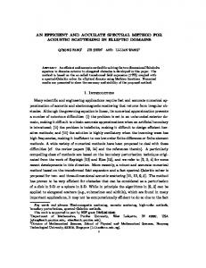
FIG. 1: (color online). Convergence of the CWDVR grid for different κ and Z values. The natural logarithm of the population decay as a function of time (in unit of laser cycle) are shown for the laser wavelength 780 nm at the peak intensity of 2 × 1014 W/cm2 . (a) Results from different CWDVR grids (κ and Z as indicated) are compared against that from FD method; (b) A magnified version of (a) for the time from 14 to 15 cycle. A.

Choice of Gauge and Convergence of the CWDVR Grid

Although different gauges describing the interacting Hamiltonian HI (t) should in principle lead to the same physical results, it is not true in practice because of different approximations and inaccurate numerical wave functions. For some approximate methods, length gauge proves to be better than the velocity gauge in some circumstances [41]. However, as discussed by Cormier and Lambropoulos [42], velocity gauge is preferable for some ab initio numerical calculations. This is connected with the fact that the canonical momentum in the velocity gauge has been reduced to a slowly varying variable since the momentum due to the strong field has been mainly removed [42]. In this case, we can avoid some widely varying variables. Especially in the present case where the wave function is expanded in terms of the spherical harmonics, much smaller L is needed for a converged result in the velocity gauge than that needed in the length gauge. In the present work, we have performed our results in the velocity gauge for H in laser fields. However, length gauge is used for H in static field and H− in laser fields. One of the reasons for the latter choice is that it is easy for us to compare our results with the 18

Log (Population)

0

-0.3

Pgrd Pinn Pmid Pwhl

-0.6

-0.9

0

20

40

Time (Cycles)

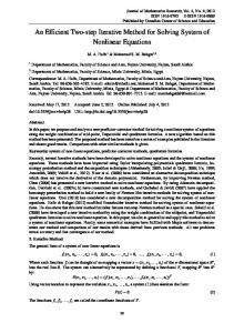
FIG. 2: The logarithm of the decay of the ground state and population within different spheres of r for H at the laser frequency ω = 0.6 a.u. and the peak intensity I0 = 4.375 × 1013 W/cm2 .

previous results. Another reason, for H − , is that the angular-momentum-dependent model potential [43] makes the form of the potential in the velocity gauge is not able to be obtained obviously [44]. Since the CWDVR grid depends on the two parameters Z and κ, one has to make sure that any calculation should be converged against changes of them. As shown in table I, the CWDVR grid for smaller κ is much coarser. At the same time, the first point of the grid is mainly decided by the value of Z. It is expected that much finer CWDVR grid will have a better representation of the Coulomb potential and the wildly driven electronic wave function by the laser field. In order to test the convergence of CWDVR grid, the multiphoton ionization of H for an infrared laser at a moderate laser intensity serves as a good example. For a hydrogenic atom, the potential is given by VC (r) = −

Z r

(65)

where Z is the nuclear charge and equals to 1 for H. For the CWDVR grids we consider in table I, we get the H ground state energy of −0.49999997 a.u. or better. In figure 1, we present the natural logarithm of the population decay within a sphere of 25 a.u. of r calculated by the FD method and by the CWDVR grids corresponding to different Z and κ. With the wavelength λ = 780 nm and peak intensity I0 = 2 × 1014 W/cm2 , the laser pusle has a 5-cycle ramping-on time and keeps constant for another 10 cycles. The maximum number of angular momentum L is taken to be 20 for a converged calculation. In 19

TABLE II: Ionization rate Γ (in s−1 ) for ionization of H by a linearly polarized laser of intensity I0 (in W/cm2 ) and frequency ω (in a.u.) . The present results (a) are compared with the previous results: (b) Chu and Cooper [45]; (c) Pont, Proulx and Shakeshaft [47]; (d) Kulander [10]. The number with parenthesis like p(q) is understood as p × 10q . ω

I0

Γa

Γb

Γc

Γd

0.55 7.00(12) 1.43(13) 1.43(13) 1.43(13) 1.4(13) 0.28 7.00(12) 3.73(11) 3.73(11) 4.0(11) 3.3(11) 4.38(13) 1.33(13) 1.33(13) 1.35(13) 1.2(13) 0.20 4.38(13) 3.74(12) 3.86(12) 4.0(12) 2.8(12) 1.75(14) 2.65(14) 2.89(14) 2.7(14) 4.0(14) 3.94(14) 6.14(14) 5.65(14) 6.0(14) 7.0(14)

the FD case, the grid spacing ∆r is taken to be 0.2 a.u., and the number of the grid point N = 750 for the maximum value of the grid point rmax = 150. The corresponding number of the r grid points used for CWDVR cases are indicated in table I. From figure 1, we conclude that our results are indeed converged to the FD difference results as κ is increased from 0.5 to 2.0. Even for the coarsest case for κ = 0.5, in which case only 56 grid points are used, the result is reasonably good. The ionization rate estimated from this curve is 4.63×1013 s−1 , which is close to the FD result 5.07×1013 s−1 and the CWDVR result 5.05×1013 s−1 for κ = 2. We also observe that, for the present case, results are not very sensitive to changing of the value of Z(for the same value of κ). However, we find that, in most of the cases that we consider later, Z = 20 is usually more preferable for its better representation of the Coulomb potential near r = 0. In practice, the ionization rate is fitted by an exponential decay of the ground state population or the decay of the total population within some sphere of r. In the present calculations, we have defined an inner sphere and a middle sphere with radius rinn = 25 and rmid = 50 a.u. respectively. The population remaining within these two spheres Pinn and Pmid , together with the probability in the ground state Pgrd and the total population in the whole box Pwhl , are recorded for each time time step. As an example, we show in figure 2 for the ionization of H at the laser frequency 0.6 a.u and peak intensity 4.375 × 1013 W/cm2 . The laser has a ramping on time of 5 cycles and keeps constant for 50 cycles. We observe

20

TABLE III: Multiphoton ionization rates of H at different laser electric field strengths Frms for different photon energies ω. Results calculated from the present method are compared with those of Chu and Cooper by a nonperturbative L2 non-Hermitian Floquet method [45]. Γ/2 (a.u.) ω

Frms = 0.01 a.u.

Frms = 0.025 a.u.

Frms = 0.05 a.u.

Frms = 0.075 a.u.

(a.u.)

Present

Ref [45]

Present

Ref [45]

Present

Ref [45]

Present

Ref [45]

0.60

0.125(-3)

0.125(-3)

0.783(-3)

0.784(-3)

0.313(-2)

0.314(-2)

0.704(-2)

0.711(-2)

0.55

0.173(-3)

0.173(-3)

0.108(-2)

0.108(-2)

0.435(-2)

0.436(-2)

0.982(-2)

0.989(-2)

0.50

0.250(-3)

0.247(-3)

0.157(-2)

0.154(-2)

0.647(-2)

0.624(-2)

0.149(-1)

0.139(-1)

0.30

0.378(-5)

0.377(-5)

0.131(-3)

0.131(-3)

0.160(-2)

0.161(-2)

0.594(-2)

0.639(-2)

0.28

0.451(-5)

0.451(-5)

0.161(-3)

0.161(-3)

0.204(-2)

0.204(-2)

0.821(-2)

0.815(-2)

0.27

0.503(-5)

0.502(-5)

0.180(-3)

0.180(-3)

0.230(-2)

0.231(-2)

0.920(-2)

0.920(-2)

0.26

0.562(-5)

0.562(-5)

0.202(-3)

0.202(-3)

0.256(-2)

0.261(-2)

0.106(-1)

0.110(-1)

0.22

0.335(-6)

0.180(-6)

0.200(-4)

0.189(-4)

0.474(-3)

0.511(-3)

0.109(-1)

0.173(-1)

0.20

0.140(-6)

0.106(-6)

0.452(-4)

0.467(-4)

0.321(-2)

0.350(-2)

0.743(-2)

0.683(-2)

0.19

0.180(-4)

0.715(-5)

0.454(-3)

0.446(-3)

0.213(-2)

0.214(-2)

0.466(-2)

0.437(-2)

0.18

0.884(-6)

0.791(-6)

0.945(-4)

0.948(-4)

0.158(-2)

0.148(-2)

0.243(-2)

0.376(-2)

that the population decay within different spheres of r are parallel lines with the line of the ground state decay. Therefore, it does not matter in this case which curve to be used for the estimation of the ionization rate. The calculated ionization 1.5658×10−3 a.u. in this way is in very good agreement with Chu and Cooper’s result 1.5672×10−3 a.u. [45]. In a similar way, we have also estimated the multiphoton ionization rate of H by the laser of wavelength 1064 nm at the peak intensity 1 × 1014 W/cm2 . The result is 2.97×1012

s−1 , which is in good agreement with an independent molecular code result 2.85×1012 s−1

in cylindrical coordinates and the FD result 2.92×1012 s−1 in spherical coordinates [46].

B.

Multiphoton Ionization of H by Intense Laser Pulses

From the above test calculations, we have seen that the present method is applicable to different laser wave lengths at different intensities. In this section, we give more rigorous 21

Log( P1s(t) )

0.0

κ=1 κ=2 κ=3 κ=4 κ=5

-0.5

-1.0

-1.5

0

100

200

300

Time (a.u.)

FIG. 3: (color online). Depletion of the ground state of H by a static electric field with the field strength 0.08 a.u.. The ground state probability is shown as a function of the field duration. Results calculated by different CDVR grids for different κ values are compared against the result calculated by FD method with ∆r = 0.1 a.u..

tests of the present method by calculating the ionization rates of H for a large number of wavelengths from very low to very high peak intensities. For all the calculations presented here, we use the CWDVR grid for κ = 1.0 and Z = 20. Therefore the number of grid point N is 72 with rmax = 151.39 a.u.. The maximum number of angular momentum L = 10 gives converged results in all the cases for the velocity gauge description of the interaction term. The parameters for the absorbing function (64) α and σ are taken to be 0.4 and 4 respectively. In table II, we compare ionization rates calculated using the present method with other theoretical results. We notice that our results agree better with those of Chu and Cooper [45] by an ab initio Floquet calculations. However, the present time-dependent method results are also in reasonable agreement with those TDSE calculations of Ref. [47] using a complex Sturmian basis and those of Ref. [10] using a FD method. The results of ω = 0.2 a.u. for intensities 1.75 × 1014 and 3.94 × 1014 W/cm2 are of less favorable agreement because high ionization rates lead to very fast decay of the ground population and thus estimations from TDSE methods become less accurate. In table III, we compare ours results with the benchmark calculations done by Chu and Cooper [45] using the ab initio nonperturbative L2 non-Hermitian Floquet method. The laser frequency ω vary from 0.6 to 0.18, which correspond to one- to three-photon ionization 22

1.00

1.0000 (a)

(b) 0.99

0.9998 0.98

P1s(t)

0.9996

0.97 0

200

400

600

1.00

0

30

60

90

1.0 (c)

(d)

0.96

0.8

0.92 0.6 0.88

0

30

60

90

0

30

60

90

FIG. 4: H ground state survival probability P1s as a function of time in static electric fields. The field strength F is taken to be: (a) 0.005; (b) 0.04; (c) 0.06; (d) 0.08 a.u.. These results are in perfect agreement with those by Durand and Paidarov´a [51] and by Scrinzi [49].

of the ground state H. Please note that E0 is connected with Frms by E0 =

√

2Frms =

p I/Iau .

(66)

Again, very good agreement are achieved for these wide ranges of laser parameters.

C.

Ionization of H by Static Electric Fields

Now let us turn to the ionization of H from the ground state by a static electric field. Excitation and ionization dynamics of atoms and molecules by static electric fields has been of great importance since the foundation of quantum mechanics [48] and continues to be of great interest of current study [49, 50, 51]. Although the long time behavior is dominated by the exponential decay of the ground state of H, large deviations from the naive exponential decay are expected because of the sudden turn-on of static electric field. Actually, the spectrum of the Hamiltonian for this system is unbounded from below. There are many resonances present. The deviation from exponential decay is expected to be large for strong fields cases [51]. However, there is a

23

substantially long time of transitory region for weak and intermediate fields as well, whose length depends on the particular field strength. In order to investigate this transitory regime, one has to make sure that the nonexponential decay indeed comes from physical dynamics rather than numerical reasons such as nonconvergence of the grid or reflection of the wave function from the edge. This point is extremely important for the static electric field case where the wave packet is driven away in one direction rather than in a oscillatory fashion as for a laser pulse case. In figure 3, we show the logarithm of the ground state probability of H by a static electric field F = 0.08 a.u. for different CWDVR grids. Note that we use the length gauge in this case for the dipole interaction. The maximum of the grid rmax for all the cases is taken to be around 150 a.u. and the corresponding number of the grid points are listed in table I. We take Z = 20 for all the CWDVR grids. In addition, the absorbing function parameters α and σ are taken to very extreme values of 0.25 and 0.4 respectively in order to avoid the reflection from the edge. For this field strength, we can get converged result only if κ > 4.0, which case the grid is dense enough for a good representation of the interaction term using the length gauge. Note that the performance of the present CWDVR is much better than the DVR method used by Dimitrovski and coworkers [52], in which case the converged result is only achieved for t ≈ 40. Therefore, one has be be very careful not to interpret the nonexponential decay for κ < 3.0 as any physical excitation and ionization dynamics [51]. Using the CWDVR κ > 4.0 and Z = 20, we have studied the short-time dynamics at other field strengths. In figure 4, we present the population decay of the ground state for different electric field strength F . For the lowest field strength F = 0.005 a.u., one observes both a small- and large-time scale regular oscillation, which implies reversible processes. For the case when F becomes 8 times of that in (a), we observe a quadratic decay in the first 8 a.u., followed by a irregular transition time before the system becomes stable after 90 a.u. or so (it will be a very slow exponential decay afterwards, with Γ ∼ 10−6 a.u.). As the field strength increases further in (c) and (d), the transitory time becomes shorter and shorter, which is followed by a purely exponential decay. The transitory regions are shown by Durand and Paidarov´a [51] to directly related to the 2s-2p resonances by inspecting the spectral density line-shape. Note that, the fast quadratic decay is present for (c) and (d) as well when the field is turned on. It is remarkable to note that the present time-dependent calculations for the entire region 24

TABLE IV: Ionization rate Γ (in a.u.) for ionization of the ground state of H by a static electric field of strength F (in a.u.). Results are compared with: (a) Scrinzi [49]; (b) Peng et al [13]; (c) Bauer and Musler [53]. F

0.06

0.08

0.1

0.5

Present 5.1509(-4) 4.5396(-3) 1.42(-2) 5.64(-1) Ref [49] 5.1508(-4) 4.5397(-3) 1.45(-2) 5.60(-1) Others 5.15(-4)b

4.55(-3)b 1.2(-2)c 5.4(-1)c

from very weak to very strong field strengths are in complete agreement with the results using the complex scaling methods [49, 51]. This is further confirmed by comparing our ionization rates fitted by an exponential decay in the region where the transitory time is over, which is shown in table IV. Also shown in this table are the results of some other time-dependent calculations [13, 53].

D.

Multiphoton detachment rates of H− by strong laser pulse

In order to show that the present method can equally apply to any atomic systems with appropriate SAE model potential, we study the in this section the multiphoton detachment of the negative ion of hydrogen. For H− , we use the angular-momentum-dependent model potential proposed by Laughlin and Chu [43]   αd 1 −2r l e − 4 W6 (r/rc ) + ul (r), VC (r) = 1 + r 2r

(67)

where j

Wj (x) = 1 − e−x ,

(68)


ul (r) = c0 + c1 r + c2 r 2 e−βr .

(69)

In the present calculations, we use the same values of parameters listed in Table I. of Ref. [43]. The length gauge is used to describe the interaction term. Please also note that, we adopt the corresponding dipole operator which includes the contribution induced on the hydrogenatom core by the outer loosely bounded electron. Instead of r, the dipole operator D in this case is given by i h αd D = 1 − 3 W3 (r/rc ) r, r 25

(70)

TABLE V: Multiphoton detachment rates of H− for 1064 nm, 1640 nm and 1908 nm at different intensities ranging from 1 × 1010 to 1 × 1012 W/cm2 . The present results from the CWDVR are compared with those of Haritos and coworkers [56] and those of Telnov and Chu [57, 58]. The detachment rate is quoted as p(q) which stands for p × 10q . Photodetachment Rate (a.u.) Intensity

1064 nm

1640 nm

1908 nm

(W/cm2 ) Present Ref [56] Ref [57] Present Ref [56] Ref [58] Present Ref [56] Ref [58] 1 × 1010

4.56(-5) 4.50(-5) 4.65(-5)

6.5(-7)

5.05(-7) 2.98(-7) 4.90(-7) 4.33(-7) 4.80(-7)

5 × 1010

2.25(-4) 2.20(-4)

7.7(-6)

6.82(-6)

1.14(-5) 1.04(-5)

8 × 1010

3.57(-4) 3.56(-4)

1.81(-5) 1.71(-5)

2.81(-5) 2.58(-5)

1 × 1011

4.43(-4) 4.43(-4) 4.53(-4) 2.79(-5) 2.63(-5) 2.78(-5) 4.27(-5) 3.98(-5) 4.37(-5)

2 × 1011

8.58(-4) 8.70(-4)

1.01(-4) 0.99(-4) 1.05(-4) 1.55(-4) 1.46(-4) 1.58(-4)

3 × 1011

1.25(-3) 1.28(-3)

2.14(-4) 2.10(-4)

4 × 1011

1.61(-3) 1.66(-3)

3.68(-4) 3.55(-4) 3.76(-4) 5.18(-4) 4.95(-4) 5.30(-4)

6 × 1011

2.24(-3) 2.38(-3)

7.62(-4) 7.19(-4)

8 × 1011

2.66(-3) 2.98(-3)

1.16(-3) 1.15(-3) 1.23(-3) 1.48(-3) 1.55(-3) 1.52(-3)

9 × 1011

2.81(-3) 3.24(-3)

1.39(-3) 1.40(-3)

1 × 1012

3.05(-3) 3.46(-3) 2.95(-3) 1.64(-3) 1.64(-3) 1.73(-3) 2.16(-3) 2.12(-3) 2.18(-3)

3.23(-4) 3.01(-4)

9.52(-4) 9.78(-4)

1.72(-3) 1.88(-3)

Use this model potential, the ground state we get is −0.027730 a.u. for all the CWDVR grids listed in table I, which is in very good agreement with the value −0.027733 a.u. calculated by Telnov and Chu [54] and with the experimental measurement −0.027716 a.u. [55]. In table V, we compare the total detachment rates of H− calculated from the present method with other theoretical calculations. We get converged results of the CWDVR grid for κ = 2 and Z = 20. It is not surprising that the requirement of the grid is less demanding for H− case than for the H in static electric field case since we have a short-range potential here. For all the laser parameters considered in table V, we get very good agreement with those results of Refs. [56] and [57, 58]. However, Telnov and Chu use the dipole moment r, which accounts for the slight differences between their results and ours. We have tested our code with the latter dipole moment,

26

we get detachment rate to be 4.51 × 10−4 a.u. instead of 4.43 × 10−4 a.u. for 1064 nm at

1 × 1011 W/cm2 . On the other hand, our results are slightly closer to those of Haritos and

coworkers [56], which are calculated by solving the time-independent Schr¨odinger equation by the nonperturbative many-electron, many-photon theory (MEMPT). This might be due to the fact that the dipole moment we use takes the core polarization effects into account.

V.

CONCLUSIONS

We have presented an accurate and efficient method of solving the time-dependent Schr¨odinger equation. Compared to the usual FD discretization scheme of the radial coordinate, the present CWDVR method needs 3-10 fewer number of grid points and treats the Coulomb singularity naturally and accurately. As examples, our method has been very successfully applied to the multiphoton ionization dynamics of both H and H− . The total ionization rates estimated from the present method are in perfect agreement with other theoretical results. We have also applied our method to investigate the short-time excitation and ionization dynamics of H in weak and strong static electric fields. The ground state survival probability and the ionization rate calculated using the present method are in full agreement with those results calculated by complex rotation method. Since the CWDVR treats the Coulomb potential accurately and needs much fewer points in r coordinate, the present methods opens the way to a more efficient treatment of many-electron atomic systems.

Acknowledgments

L.Y.P. appreciates helpful discussions with Profs. D.A. Telnov and S.I. Chu about gauge choice of H− and communications with Prof. R.B. Sidje about application of the package “Expokit”. This research is partially supported by NSF and DOE.

[1] T. Brabec and F. Krausz, Rev. Mod. Phys. 72, 545 (2000). [2] M. Protopapas, C. H. Keitel and P. L. Knight, Rep. Prog. Phys. 60, 389 (1997). [3] (a) P. Agostini and L. F. DiMauro, Rep. Prog. Phys. 67, 813 (2004); (b) A. Scrinzi, et al, J. Phys. B: At. Mol. Opt. Phys. 39, R1 (2006).

27

[4] (a) A. F¨ohlisch, et al, Nature 436, 373 (2005); (b) M. Wickenhauser, et al, Phys. Rev. Lett. 94, 023002 (2005); (c) K. Ohmori, et al, Phys. Rev. Lett. 96, 093002 (2006). [5] M. V. Ammosov, N. B. Delone and V. P. Krainov, Sov. Phys. JETP, 64, 1191 (1986). [6] A. Becker and F. H. M. Faisal, J. Phys. B: At. Mol. Opt. Phys. 38, R1 (2005). [7] S. I. Chu and D. A. Telnov, Phys. Rep. 390, 1 (2004). [8] P. G. Burke and V. M. Burke, J. Phys. B: At. Mol. Opt. Phys. 30, L383 (1997). [9] M. A. L. Marques and E. K. U. Gross, Annu. Rev. Phy. Chem. 55, 427 (2004) [10] K. C. Kulander, Phys. Rev. A 35, 445 (1987). [11] (a) H. G. Muller, Laser Physics 9, 138 (1999); (b) D. Bauer and P. Koval, Comput. Phys. Commun. 174, 396 (2006). [12] (a) E. S. Smyth, J. S. Parker and K. T. Taylor, Comput. Phys. Commun. 114, 1 (1998) ; (b) K. T. Taylor,et al, Phys. Script. T110, 154 (2004). [13] L. Y. Peng, et al, J. Chem. Phys. 120, 10046 (2004). [14] K. J. Meharg, J. S. Parker and K. T. Taylor, J. Phys. B: At. Mol. Opt. Phys. 38, 237 (2005). [15] (a) S. Qu and J. H. Eberly, Phys. Rev. A 44, 5997 (1991); (b) M. S. Pindzola, P. Gavras and T. W. Gorczyca, Phys. Rev. A 51, 3999 (1995); (c) V. V´eniard, R. Ta¨ieb and A. Maquet, Phys. Rev. A 60, 3952 (1999); (d) C. Ruiz, L. Plaja and L. Roso, Phys. Rev. Lett. 94, 063002 (2005). [16] (a) J. von Milczewski, D. Farrelly and T. Uzer, Phys. Rev. Lett. 78, 2349 (1997); (b) A. Gordon, R. Santra and F. X. K¨ artner, Phys. Rev. A 72, 063411 (2005). [17] G. L. Ver Steeg, K. Bartschat and I. Bray, J. Phys. B: At. Mol. Opt. Phys. 36, 3325 (2003). [18] (a) B. I. Schneider and N. Nygaard, Phys. Rev. E 70, 056706 (2004); (b) H. Kono, et al, J. Comput. Phys. 130, 148 (1997); (c) G. Czako, et al, J. Chem. Phys. 122, 024101 (2005). [19] (a) D. Comtois, et al, J. Phys. B: At. Mol. Opt. Phys. 38, 1923 (2005); (b) A. Rudenko, et al, J. Phys. B: At. Mol. Opt. Phys. 38, L191 (2005). [20] D. O. Harris, G. G. Engerholm and W. D. Gwinn, J. Chem. Phys. 43, 1515 (1965). [21] A. S. Dickinson and P. R. Certain, J. Chem. Phys. 49, 4209 (1968). [22] (a) J. V. Lill, G. A. Parker and J. C. Light, Chem. Phys. Lett. 89, 483 (1982); (b) R. W. Heather and J. C. Light, J. Chem. Phys. 79, 147 (1983); (c) J. C. Light, I. P. Hamilton and J. V. Lill, J. Chem. Phys. 82, 1400 (1985). [23] (a) J. C. Light and T. Carrington Jr., Adv. Chem. Phys. 114, 263 (2000); (b) H. S. Lee and J.

28

C. Light, J. Chem. Phys. 120, 4626 (2004); (c) J. Tennyson, et al, Comput. Phys. Commun. 163, 85 (2004). [24] (a) D. T. Colbert and W. H. Miller, J. Chem. Phys. 96 1982 (1992); (b) J. Echave and D. C. Clary, Chem. Phys. Lett. 190, 225 (1992); (c) R. G. Littlejohn et al, J. Chem. Phys. 116, 8691 (2002); (d) B. I. Schneider, Phys. Rev. A 55, 3417 (1997); (e) T. N. Rescigno, D. A. Horner, F. L. Yip, and C. W. McCurdy Phys. Rev. A 72, 052709 (2005); (f) B. I. Schneider and L. A. Collins, J. Non-Cryst. Solids, 351, 1551 (2005). [25] (a) D. Baye and P. H. Heenen, J. Phys. A: Math. Gen., 19, 2041 (1986); (b) V. Szalay, J. Chem. Phys. 99, 1978 (1993) [26] J. P. Boyd, Chebyshev and Fourier Spectral Methods, 2nd ed. (Dover, New York, 2000), ch 5. [27] G. Szeg¨ o, Orthogonal Polynomials (Am. Math. Soc., Providence, Rhode Island, 1939). [28] Handbook of Mathematical Functions, ed. by M. Abramowitz and I. A. Stegun (Dover, New York, 1965). [29] C. Schwartz, J. Math. Phys. 26, 411 (1985). [30] K. M. Dunseath, J. M. Launay, M. Terao-Dunseath and L. Mouret, J. Phys. B: At. Mol. Opt. Phys. 35 3539 (2002). [31] D. A. Varshalovich, A. N. Moskalev and V. K. Khersonskii, Quantum Theory of Angular Momentum (World Scientific, Singapore, 1988). [32] A. R. Barnett, Comput. Phys. Commun., 27, 147 (1982). [33] M. D. Feit and J. A. Fleck Jr., J. Comput. Phys. 47, 412 (1983). [34] H. Tal-Ezer and R. Kosloff, J. Chem. Phys. 81, 3967 (1984). [35] H. X. Qiao, et al, Phys. Rev. A 65, 063403 (2002). [36] (a) T. J. Park and J. C. Light, J. Chem. Phys. 85, 5870 (1986); (b) C. S. Guiang and R. E. Wyatt, Int. J. Quantum Chem. 67, 273 (1998); (c) M. Hochbruck and C. Lubich, SIAM J. Numer. Anal., 34, 1911 (1997); (d) M. Hochbruck, C. Lubich and H. Selhofer, SIAM J. Sci. Comput., 19, 1552 (1998). [37] (a) C. Leforestier, et al, J. Comput. Phys. 94, 59 (1991); (b) T. N. Truong, et al, J. Chem. Phys. 96, 2077 (1991); (c) C. Moler and C. Van Loan, SIAM REVIEW, 45, 3 (2003); (d) A. Castro, M. A. L. Marques and A. Rubio, J. Chem. Phys. 121, 3425 (2004). [38] Y. Saad, Iterative Methods for Sparse Linear Systems, 2nd ed. (SIAM, Philadelphia, 2003), ch 6.

29

[39] R. B. Sidje, ACM Trans. Math. Software, 24, 130 (1998). [40] (a) U. V. Riss and H. D. Meyer, J. Phys. B: At. Mol. Opt. Phys. 28, 1475 (1995); (b) J. G. Muga, et al, Phys. Rep. 395, 357 (2004); (c) R. Lefebvre, M. Sindelka and N. Moiseyev, Phys. Rev. A 72, 052704 (2005); (d) O. Shemer, D. Brisker and N. Moiseyev, Phys. Rev. A 71, 032716 (2005); (e) S. Scheit,et al, J. Chem. Phys. 124, 034102 (2006). [41] T. K. Kjeldsen and L. B. Madsen, Phys. Rev. A 71, 023411 (2005). [42] E. Cormier and P. Lambropoulos, J. Phys. B: At. Mol. Opt. Phys. 29 1667 (1996). [43] C. Laughlin and S. I. Chu, Phys. Rev. A 48, 4654 (1993). [44] D. A. Telnov and S. I. Chu, J. Phys. B: At. Mol. Opt. Phys. 28 2407 (1995). [45] S. I. Chu and J. Cooper, Phys. Rev. A 32, 2769 (1985). [46] L. Y. Peng, et al, J. Phys. B: At. Mol. Opt. Phys. 36 L295 (2003). [47] M. Pont, D. Proulx and R. Shakeshaft, Phys. Rev. A 44, 4486 (1991). [48] L. D. Landau and E. M. Lifshitz, Quantum Mechanics, 2nd (Pergamon, Oxford, 1965). [49] A. Scrinzi, Phys. Rev. A 61, 041402 (2000). [50] (a) S. Geltman, J. Phys. B: At. Mol. Opt. Phys. 33, 4769 (2000); (b) A. A. Kudrin and V. P. Krainov, Laser Physics 13, 1024 (2003); (c) G. V. Dunne and C. S. Gauthier, Phys. Rev. A 69, 053409 (2004); (d) R. M. Cavalcanti1, P Giacconi and R Soldati, J. Phys. A: Math. Gen. 36, 12065 (2003). [51] P. Durand and I. Paidarova, Eur. Phys. J. D 26, 253 (2003). [52] D. Dimitrovski, et al, J. Phys. B: At. Mol. Opt. Phys. 36, 1351 (2003). [53] D. Bauer and P. Mulser, Phys. Rev. A 59, 569 (1999). [54] D. A. Telnov and S. I. Chu, J. Phys. B: At. Mol. Opt. Phys. 37, 1489 (2004). [55] K. R. Lykke, K. K. Murray and W. C. Lineberger, Phys. Rev. A 43, 6104 (1991). [56] C. Haritos, T. Mercouris and C. A. Nicolaides, Phys. Rev. A 63, 013410 (2000). [57] D. A. Telnov and S. I. Chu, J. Phys. B: At. Mol. Opt. Phys. 29, 4401 (1996). [58] D. A. Telnov and S. I. Chu, J. Phys. B: At. Mol. Opt. Phys. 59, 2864 (1999).

30