porate total generalized variation (TGV) and shearlet trans- form to efficiently produce high quality images from com- pressive sensing MRI data, i.e., incomplete ...
2013 IEEE 10th International Symposium on Biomedical Imaging: From Nano to Macro San Francisco, CA, USA, April 7-11, 2013
AN EFFICIENT COMPRESSIVE SENSING MR IMAGE RECONSTRUCTION SCHEME Jing Qin, Weihong Guo Case Western Reserve University Department of Mathematics 10900 Euclid Ave, Cleveland, OH 44106 ABSTRACT
Φ is usually chosen to be total variation and/or wavelet. Unlike wavelet transform limited to 1D isotropic representation, shearlet transform has been proven optimal in sparsely representing images with directional information [4]. For any function in L2 (R2 ), the N largest term approximation using shearlet transform has error O((log N )3 /N 2 ) while O(1/N ) for wavelet transform. To reduce the staircase effects of TV and efficiently represent images with rich anisotropic features, we combine TGV and shearlet transform. Various numerical experiments show that the combination works better than TGV or shearlet only, and is significantly better than some existing reconstruction approaches using TV and/or wavelet. The rest of this paper is organized as follows. We start with a brief review on TGV and shearlet transform in Section 2 and present the proposed model and algorithm in Section 3. Section 4 shows numerical simulation results. Finally, conclusions are drawn in Section 5.
Compressive sensing (CS) has great potential to reduce imaging time. It samples very few linear projections, and exploits sparsity or compressibility to reconstruct images from the measurements. Medical and most natural images usually contain various fine features, details and textures. Widely used total variation (TV) and wavelet sparsity are not so effective in reconstructing these images. We propose to incorporate total generalized variation (TGV) and shearlet transform to efficiently produce high quality images from compressive sensing MRI data, i.e., incomplete spectral Fourier data. The proposed model is solved by using split Bregman and primal-dual methods. Numerous numerical results on various data corresponding to different sampling rates and noise levels show the advantage of our method in preserving various geometrical features, textures and spatially variant smoothness. The proposed method consistently outperforms related competitive methods and shows greater advantage as sampling rate goes lower.
2. PRELIMINARIES
Index Terms— compressive sensing, total generalized variation, primal dual, split Bregman, MRI
In this section, we briefly review the concepts and properties of TGV and shearlet transform. TGV. Different from TV that approximates image intensities by piecewise constant functions, TGV uses piecewise polynomials with flexible degrees. Thus it does not lead to staircase effects as in TV but creates piecewise smooth intensities. Let Ω be a non-empty, open and connected set in Rd and α = (α0 , α1 ) a positive multi-index. The second order TGV with weight α for�u ∈ L1loc (Ω) is� defined as � � u div2 w dx � w ∈ Cc2 (Ω, S d×d ), TGV2α (u) = sup � Ω (1) �w�∞ ≤ α0 , �divw�∞ ≤ α1 where S d×d is the space of 2nd order d × d symmetric matrices. It can be generalized to higher order TGV. Introducing the indicator functional IK defined as IK (x) = 0 if x ∈ K and ∞ or else, and using the fact I{0} (x) = − miny �y, x�, the discretized TGV2α can be written as
1. INTRODUCTION Compressive sensing (CS) reduces imaging time by sampling much fewer measurements than that desired by the NyquistShannon sampling theorem [1]. CS reconstruction utilizes the sparsity or compressibility of the signals to reconstruct them (cf. the pioneering work [2, 3]). Most of the existing CS reconstruction methods are effective for piecewise constant images, but not for most medical and natural images that are piecewisely smooth. Assume u ¯ ∈ Cn is the underlying image of interest, the incomplete measurement is b = Ψ¯ u or Ψ¯ u + r where r is noise, Ψ ∈ Cm×n with m � n is called sensing (sampling) matrix. To solve the underdetermined system, one assumes u ¯ itself or under some transform Φ is sparse/compressible. A popular approach to reconstructing u ¯ is to solve the �1 optimization problem min λ�Φu�1 + 12 �Ψu − b�2 that is more computationally feasible and equivalent to its �0 counterpart under some conditions (e.g. [2]). The sparsifying transform
978-1-4673-6455-3/13/$31.00 ©2013 IEEE
TGV2α (u) = min max�∇u − p, v� + �E(p), w�
p (v,w) (2) − I{�·�∞ ≤α0 } (w) − I{�·�∞ ≤α1 } (v), where u, v, w belong to the respective suited spaces of functions defined on the discretized image domain and E is an
306
where the shrinkage is defined by shrink(v, δ) = sgn(v). ∗ max{|v| − δ, 0} with sgn(x) : Cn → Cn whose components are sign functions and all the arithmetic operations are implemented componentwisely. For the second subproblem which belongs to min-max problems, we adopt primal-dual algorithm and derive the closed-form solution as follows. Let
operator. See [5] for more details. Shearlet transform. Given any ψ ∈ L2 (R2 ), the affine − 12 −1 system is generated by � {ψast √ =� | det Mas | ψ(Mas (x − a −√ as t))}, where Mas = . Then the affine function a 0 ψast is called shearlet and depends on three parameters: scale a, shear s and translation t. Shearlet transform of any given f ∈ L2 (R2 ) based on ψ is defined as SHα ψ (f )(a, s, t) = �f, ψast �. Discrete shearlet transform can be efficiently computed using fast Fourier transform. More details can be found for instance in [4, 6].
E(u) =
then the second subproblem reads as minu E(u)+TGV2α (u). Next we derive the resolvent (I + η∂E)−1 required in the primal step. Considering the following minimization prob2 lem minu �u − u ¯�2 /2+ηE(u), we get the associated normal equation as N � ∗ MH MHj )u = (I + ηβFp∗ Fp + ηλτ j
3. PROPOSED MODEL AND ALGORITHM For the convenience of discussion, we assume that the available MRI data is partial Fourier transform of the underlying image of interest, i.e., Ψ = Fp = P F which is product of the diagonal selection matrix P ∈ Rm×n and one Fourier transform related unitary matrix F ∈ Cn×n . Combining shearlet and the second order TGV, we propose the following model: N � β 2 �SHj (u)�1 + TGV2α (u) + �Fp (u) − b�2 min λ u 2 j=1
j=1
u ¯ + ηβFp∗ b + ηλτ
N �
∗ MH (sj − tj ). j
j=1
To circumvent the expensive computation of the inverse of large matrices, we rewrite the normal equation after multiplying both sides by F and use the properties of Fourier transform matrix F ∗ F = I and the fact that circulant matrices can be diagonalized under the Fourier transform. Then we get the solution in matrix form as �N
� Fu ¯ + ηβb + ηλτ j=1 Hj∗ . ∗ F(sj − tj ) −1 u=F �N 1 + ηβP T P + ηλτ j=1 |Hj |.2 (3) where the division is componentwise. We list our algorithm combining alternating minimization scheme and primal-dual method as below:
where SHj (u) is the j-th subband of Shearlet transform of u. We adopt the approach in [6] and use Fourier and inverse Fourier transform to compute shearlet transform. SHj (u) can be efficiently implemented as componentwise multiplication with a wedge shaped 0-1 mask function Hj in frequency domain, namely SHj (u) = F ∗ diag(vec(Hj ))F u := MHj u. The proposed model is not trivial to solve due to nondifferentiability of many �1 terms and the complex definition of the TGV term. We use split Bregman method to handle the non-differentiability of the �1 terms and use primal-dual method to deal with TGV. We first introduce the auxiliary variables sj ∈ Cn and enforce them to be close to SHj (u) by adding quadratic penalty. N � τ 2 (�sj �1 + �sj − SHj (u) − tj �2 ) + TGV2α (u) min λ u 2 j=1 β 2 + �Fp (u) − b� 2 where tj ’s are updated by Bregman iterations. We then decompose the original problem into two sets of subproblems and apply the alternating minimization scheme as follows ⎧ τ 2 ⎪ min �sj �1 + �sj − SHj (u) − tj �2 , j = 1, . . . , N ⎪ ⎪ sj 2 N ⎪ ⎪ β λτ � ⎨ 2 2 �sj − SHj (u) − tj �2 min �Fp (u) − b�2 + u 2 2 ⎪ j=1 ⎪ ⎪ + TGV2α (u) ⎪ ⎪ ⎩ tj ← tj + γ(SHj (u) − sj ), j = 1, . . . , N. The first set of subproblems can be solved by applying the shrinkage operator sj = shrink(SHj (u) + tj , 1/τ ),
N λτ � β 2 2 �Fp u − b�2 + �sj − SHj u − tj �2 , 2 2 j=1
Algorithm 1 TGV based image reconstruction algorithm 1. Choose σ, η > 0. 2. Initialize u0 , p0 , v 0 , s0i , t0i , i = 1, . . . , N . 3. For n = 0, 1, 2, . . ., run the following computations = shrink(SHj (un ) + tni , 1/τ ), sn+1 j v
n+1
w
n+1
n
n
= Pα0 (wn + σE(¯ pn ))
un+1 = (id + η∂E)−1 (un + η divv n+1 ) p
n+1
= p + η(v
n+1
n+1
u ¯
n+1
p¯
j = 1, . . . , N
= Pα1 (v + σ(∇¯ u − p )) n
n
=u =p
n+1
n+1
n+1
−u )
n+1
− pn )
+ θ(u + θ(p
+ divw
n+1
(Use (3))
)
n
tn+1 = tnj + γ(SHj un+1 − sn+1 ), j = 1, . . . , N. j j � � n n+1 � ≤ tol, it returns un+1 and stops If �u − u 4. EXPERIMENTS In this section, we test our algorithm on a variety of images and compare them with three recently proposed algorithms:
j = 1, . . . , N,
307
Fig. 2. Reconstruction errors. From left to right: proposed, RecPF, EdgeCS. SNR’s are: 27.41, 23.28, 23.51 respectively. 30
Fig. 1. Axial brain MR image reconstruction. First row from left to right: ground truth and our result. Second row from left to right: results obtained by RecPF and EdgeCS.
25
SNR
20
15
10
reconstruction from partial Fourier data (RecPF) [7], edge guided compressive sensing reconstruction (EdgeCS) [8] and TGV based MRI reconstruction (TGV-L2 ) [9]. The comparison with RecPF and EdgeCS shows the advantage of TGV over TV, and the comparison with TGV-L2 shows that it is necessary to combine shearlet with TGV. All the quantitative comparisons are based on signal-to-noise ratio (SNR) defined �utrue �22 as 10 log10 �u−u 2 . The convergence of the proposed altrue �2 √ gorithm is guaranteed by ση < 1/16, 0 < τ, ρ < ( 5+1)/2, θ = 1, γ > 0, ν > 0. β and λ depend on the TGV/shearlet transform sparsity of the underlying image and the noise/error level in the measurements. We set σ = 0.05, η = 0.1, τ = ρ = 0.2, γ = ν = 10−2 . We fix α = 10−3 and β = 102 for all noiseless data and raise a little as noise level increases. We use three-scale shearlet transform which has 13 subbands. The tests were performed on simulated data and real in vivo data. First we test the simulated k-space data of one noise-free axial slice of T1-weighted brain MRI series with uniform intensity obtained from brainweb. We tested the three methods with 40 radial sampling lines, namely 19.92% sampling rate. In Fig. 1, we show the results obtained by each method and their respective zoomed-in patches to compare the local recovery performance. We also take the difference between the ground truth and the reconstructed image for each method and display the inverted residue images in FIG. 2. One can see that the proposed method provides clearer features and higher accuracy. RecPF oversmoothes the details with relatively small intensity variations. EdgeCS highlights certain intensity jumps but neglects the weak edges and loses natural transition between boundaries and smooth areas. We also tested various number of radial sampling lines with the same parameter setting. Based on the quantitative results in Fig. 3, the proposed method shows greater advantage over the other two when the available data is reduced. Next we will show the benefits of our proposed model to reconstruct texture images due to shearlet transform. The test image is Barbara image with various texture patterns and a lot more details. The results of the proposed and three
5 0.05
Proposed RecPF EdgeCS 0.1
0.15 sampling rate
0.2
0.25
Fig. 3. Plots of SNR versus sampling rate for each method. other methods from 70 radial sampling lines (sampling rate 14.74%) are listed in Fig. 4, where we zoomed in one patch of table cloth. Our proposed method is able to recover largely the directional textures while the other three methods result in blurry textures or lost of textures. The consistent performance is illustrated in Fig. 5 using different sampling rates, where the proposed algorithm significantly outperforms. In FIG. 6 and FIG. 7, we apply our proposed algorithm on the 256 × 256 in vivo brain image provided by medical school of CWRU. Here we use the random sampling with a 40×40 box fixed in low frequency area. By changing the random sampling rate given the same fixed low frequencies, we compare our proposed method with TGV-L2 , Shearlet L1 -L2 , RecPF (TV-wavelet L1 -L2 ) and EdgeCS in terms of relative error and SNR. And the results are illustrated in FIG. 7. 5. CONCLUSION We combined shearlet and TGV to reconstruct high quality images from few MR compressive sensing measurements. The model is not trivial to solve. We utilize split Bregman and primal-dual optimization approaches to get the solutions. In each inner iteration, there is a closed-form solution for each subproblem. Numerical results show the consistent excellence and robustness of the proposed algorithm. Various comparisons prove that combing shearlet and TGV works better than TGV only, and better than any TV/wavelet based approaches. Furthermore, our proposed method shows great advantage in preserving diverse texture patterns of the image during the reconstruction. 6. ACKNOWLEDGMENTS The authors thank the partial support from Case Western Reserve University ACES+ advance opportunity funds. We
308
32 30 28 26
SNR
24
Proposed TGVL2 L1L2 RecPF EdgeCS
22 20 18 16 14 12 0.1
0.2
0.3 0.4 sampling rate
0.5
0.6
Fig. 7. Plots of SNR versus sampling rate for reconstruction of in vivo medical data. also thank Kristian Bredies (University of Graz) for providing codes of TGV2 based image denoising, and Nicole Seiberlich (Biomedical Engineering Department, Case Western Reserve University) for providing the in vivo compressive sensing MR data. Thanks also go to the reviewers who help improve the presentation of the paper.
Fig. 4. Barbara image reconstruction. First row from left to right: ground truth and our result. Second row from left to right: results by RecPF and EdgeCS. Third row: result by TGV-L2 .
7. REFERENCES [1] C. E. Shannon, “Communication in the presence of noise,” Proc. Institute of Radio Engineers, vol. 37, no. 1, pp. 10–21, 1949.
17 16 Proposed RecPF EdgeCS TGVL2
15
SNR
14
[2] E. Cand`es and T. Tao, “Near optimal signal recovery from random projections: universal encoding strategies,” IEEE Transactions on Information Theory, vol. 52, no. 1, pp. 5406–5425, 2006.
13 12 11 10 9 8 0.08
0.1
0.12
0.14 0.16 sampling rate
0.18
0.2
0.22
[3] D. Donoho, “Compressed sensing,” IEEE Transactions on Information Theory, vol. 52, pp. 1289–1306, 2006.
Fig. 5. Plots of SNR versus sampling rate for Barbara image reconstruction.
[4] K. Guo, G. Kutyniok, and D. Labate, “Sparse multidimensional representations using anisotropic dilation and shear operators,” Wavelets und Splines (Athens, GA, 2005), Nashboro Press, Nashville, TN, pp. 189–201, 2006. [5] K. Bredies, K. Kunisch, and T. Pock, “Total generalized variation,” SIAM J. Imaging Sci., vol. 3(3), 2010.
Ground truth
RecPF
Proposed
[6] S. H¨ auser, “Fast finite shearlet transform: a tutorial,” arXiv, vol. 1201.1773v1, 2011. [7] J. Yang, Y. Zhang, and W. Yin, “A fast alternating direction method for TVL1-L2 signal reconstruction from partial fourier data,” Selected Topics in Signal Processing, IEEE Journal of, vol. 4(2), pp. 288–297, 2010.
EdgeCS
[8] W. Guo and W. Yin, “Edge guided reconstruction for compressive imaging,” SIAM J. Imaging Sci., vol. 5(3), pp. 809–834, 2012. [9] F. Knoll, K. Bredies, T. Pock, and R. Stollberger, “Second order total generalized variation (TGV) for MRI,” Magnetic Resonance in Medicine, vol. 65(2), pp. 480–491, 2011.
L1 -L2 TGV-L2 Fig. 6. Reconstruction of in vivo medical data.
309