approach for mobile nodes using wireless and ranging devices. We consider scenarios where node mobility follows stop-and-go behavior; we can then utilize ...
An Efficient Localization Algorithm Focusing on Stop-and-Go Behavior of Mobile Nodes Takamasa Higuchi† Sae Fujii† Hirozumi Yamaguchi†,‡ Teruo Higashino†,‡ † Graduate School of Information Science and Technology, Osaka University 1-5 Yamadaoka, Suita, Osaka 565-0871 Japan ‡ Japan Science and Technology Agency, CREST {t-higuti,s-fujii,h-yamagu,higashino}@ist.osaka-u.ac.jp Abstract—This paper presents a cooperative localization approach for mobile nodes using wireless and ranging devices. We consider scenarios where node mobility follows stop-and-go behavior; we can then utilize the different movement states of nodes as an input to our localization approach. In the proposed method, each node autonomously finds among its surrounding nodes the ones that do not seem to move, and treats them as static nodes. Only nodes that are deemed static are then used as reference points for position estimation. Furthermore, each node adjusts its localization frequency automatically according to its estimated velocity. Performance evaluation results based on a realistic sensor model and actual mobility traces show that our method could achieve sufficient accuracy and efficiency for an exhibition scenario where people need to be tracked.
I. I NTRODUCTION In recent years, location-aware services such as car navigation systems and pedestrian navigation applications on cell phones have spread rapidly. However, to provide realtime position information to people indoors, e.g., exhibition patrons, visitors of museums, and customers at shopping malls is still a big challenge. Instead of fully relying on fixed infrastructure that incurs high installation and maintenance cost, “cooperative localization” [1] techniques may be employed where distance information between neighboring nodes is used in estimating their location. To accomplish acceptable accuracy in cooperative localization of mobile nodes, frequency of position updates should be sufficiently high. Otherwise, position errors of mobile nodes will be accumulated as they move, which seriously degrades the estimation accuracy of other nodes when the nodes are used as reference points. On the other hand, localization frequency should be reduced because consumption of battery and network resources generally increases with the total number of localization attempts. Several methods such as [2] have been investigated for cooperative localization, but to the best of our knowledge, none of them tackles these problems. A detailed survey will be given in Section II. This paper proposes a novel cooperative algorithm to localize mobile nodes. Each mobile node is assumed to have both an ultrasound (or similar) ranging device and a wireless device to allow TDoA (Time Difference of
Arrival) distance measurement between mobile nodes. Then nodes can estimate their location based on the distance information to a reasonable number of anchors. Utilizing “stop-and-go” behavior of mobile nodes, which is generally followed by people at exhibitions, we achieved high tracking performance with a reduced number of localization attempts. To observe the performance of the presented method in realistic applications, 12 students were asked to play the role of presenters and audiences in a conference poster session. Thus we were able to obtain actual mobility traces. In addition, in our evaluation we are using a realistic ultrasound sensor model (for ranging) which was established by measurements on real devices. The experimental results using these traces and the sensor model show an average error for our method to be around 0.3m, which is sufficiently accurate. II. R ELATED W ORK For indoor positioning, most techniques rely on fixed infrastructure. For instance, RFID-tags have often been used [3], [4]. However, due to their limited radio range, a number of tags have to be embedded, which incur huge cost in wide indoor space such as an exhibition hall. Some methods utilize “signature” of radio signals. Wi-Fi-based methods [5], [6] employ a learning phase where signal strength from multiple stations at each position is recorded to build a “radio map”, and identify the location of mobile nodes by finding the best-match during localization. Cellular-phone based methods such as Calibree [7] use connectivity and signal strength from GSM cell towers to provide relatively rough position at a reasonable cost. Calibree estimates relative distance between mobile nodes based on difference of the GSM signature. For positioning with limited infrastructure, network-based localization has been considered in WSNs, MANETs and VANETs. Some method like [8], [9] assume collection of network information at a point for position estimation. SISR [10] proposed an error-tolerant localization algorithm introducing an improved residual function for the least squares method. However, they incur information collection cost and
delay, which is not preferable for real-time position estimation of mobile nodes frequently changing their location. Some other methods use estimated positions of neighboring nodes. In DOLPHIN [1], each node uses both anchors and neighboring nodes that have already been localized as reference points. Nodes can immediately estimate their positions by trilateration whenever they obtain distance information from a sufficient number of reference points, and this is continued until all nodes are localized. In [11], [12], “confidence” of estimated positions is introduced to improve position accuracy. Since they have not considered mobility of nodes that accumulate position errors as they move, they cannot be directly applied to mobile scenarios. Some cooperative localization methods have been designed for fully-distributed mobile ad hoc networks. TRADE [2] proposes real-time localization in a fully distributed manner. Mobile nodes estimate and update their trajectory information based on neighboring nodes’ trajectory information and wireless connectivity information. [13] proposes a distributed algorithm based on Sequential Monte Carlo method, in which the estimated position is regarded as a probability distribution represented by a collection of sample points. Uncertainty of the estimated position due to the noisy measurements is estimated from the variance of the sample points and utilized to mitigate error propagation. WMCL [14] also proposes a Sequential Monte Carlo-based algorithm, which uses estimated positions of neighbor nodes to reduce the computational cost and improve accuracy. Although these methods are capable of tracking mobile nodes, they commonly suffer high localization frequency issue as mentioned in section I. Compared with a number of novel positioning and localization methods, our contribution is summarized as follows. Firstly, we propose a novel distributed cooperative localization algorithm for mobile nodes. To pursue the best trade-off between localization frequency and estimation accuracy, we focus on scenarios where mobile nodes exhibit “stop-andgo” behavior (visitors stopping at exhibitions in museums, customers stopping at shelves in supermarkets, etc.). The key idea of our algorithm is that each mobile node estimates its position based on the estimated positions of surrounding nodes that have remained at their previous positions since the last localization round. Because their positions have not changed, they can be considered up-to-date and thus the position error accumulated due to mobility does not propagate to other nodes. Detection of nodes’ movement is done during the localization process using only distance information. Moreover, each node will autonomously adjust its localization frequency according to its estimated velocity. This can reduce “redundant” localization that is not expected to contribute to position accuracy improvement. Secondly, we conducted experiments assuming a real application with real trace data and real ranging devices as well as extensive simulations. Existing distributed cooperative
A1�(x1,�y1)
v1�=�0.0�m/s
d1
A0�
A0�(x0,�y0)
A5�(x5,�y5)
v5�=�0.0�m/s
Figure 1.
v2�=�0.0�m/s
d2
movement
v0�=�1.1�m/s
A2�(x2,�y2)
measured� distance
d5
d3 A3�(x3,�y3)
v3�=�0.0�m/s
A4�(x4,�y4)
v4�=�1.0�m/s
Concept of the Proposed Algorithm.
algorithms such as TRADE [2] and WMCL [14] do not consider such realistic cases. From these results, we show the applicability of our method to real world situations. III. P RELIMINARIES 2-dimensional localization requires distance information from at least three reference points. Instead of obtaining distance information to many anchor nodes, our method uses estimated positions of neighboring nodes as reference points. We will refer to such semi-mobile reference points as semi-anchors. Thus we assume that three or more anchors are deployed at known positions in a target area, and that all nodes have ad hoc communication and range measurement faculties. For range measurement, this paper assumes a Time Difference of Arrival (TDoA) technique as provided by ultrasound devices. A node simultaneously transmits RF and ultrasound signals to allow a receiver node to calculate the time difference of two signals to estimate the distance. Hence, nodes are equipped with transmitters and receivers of ultrasound signals in addition to a wireless communication technology such as IEEE802.15.4. On account of its accurate ranging capability, ultrasonic ranging provides precise, robust indoor positioning, and thus has been commonly-used in indoor localization methods such as DOLPHIN [1] and Cricket [15]. Since an ultrasound transmitter has a directional range pattern, we assume that each node has several ultrasound transmitters and receivers which are arranged radially to achieve the omni-directional range pattern. We note that although we used ultrasonic transducers in our experiments, our algorithm also works with wireless radio ranging devices such as IEEE 802.15.4a. IV. A LGORITHM D ESCRIPTION A. Overview For localizing a node, our algorithm identifies “temporarily stopping nodes” from its neighbors to choose appropriate semi-anchors. This is also effective to reduce localization frequency, because we do not have to localize such temporarily stopping nodes before they move again. Based on the idea, the outline of the algorithm is explained below. Each node 𝐴𝑖 holds position (𝑥𝑖 , 𝑦𝑖 ) and speed 𝑣𝑖 as well as its “state,” which is any of static, moving, and unknown. Anchor nodes are stationary and thus always have static state, whereas the other nodes are initially in unknown state. Node 𝐴𝑖 estimates its position, speed, and state at a
certain interval, which is adapted to the estimated speed. The algorithm of interval adaptation is given in Section IV-C. When 𝐴𝑖 performs localization, it simultaneously transmits RF and ultrasound signals to let its neighboring nodes perform TDoA distance estimation. Then neighboring node 𝐴𝑗 immediately sends a reply message including the estimated distance and 𝐴𝑗 ’s current position to 𝐴𝑖 , only if 𝐴𝑗 is in static state. Then 𝐴𝑖 can perform localization using the neighboring nodes’ positions as reference points. A problem is that the nodes in static state may actually be moving. It may often happen since the state of a node is updated only when it is localized. To prevent such nodes that may have large position error from being chosen as semianchors, 𝐴𝑖 estimates 𝐴𝑗 ’s correct state using the received distance and position information, and then uses 𝐴𝑗 as a semi-anchor only if 𝐴𝑗 seems to be actually stopping. This process is explained in Section IV-B. If three or more anchors or semi-anchors are found, 𝐴𝑖 estimates its position by the least squares method. After that, the state of 𝐴𝑖 is set to static if the estimated position is close to the old position, otherwise moving. We note that in the case that two or less static nodes have replied to 𝐴𝑖 , nodes in moving state also reply to 𝐴𝑖 . If node 𝐴𝑖 finds that 𝐴𝑗 in static state is actually moving, 𝐴𝑖 notifies 𝐴𝑗 of the fact. Then 𝐴𝑗 changes its state to moving and immediately attempts localization. Fig. 1 shows the localization process of 𝐴0 . Based on its estimated speed, 𝐴0 innovates its localization process by range measurement signal. Then nodes 𝐴1 , 𝐴2 , 𝐴3 and 𝐴5 in static state reply with distance and position information. B. State Decision Process This section explains how to choose semi-anchors from neighbors in static state on localizing 𝐴𝑖 . Hereafter, the measured distance from 𝐴𝑖 to a neighbor 𝐴𝑗 is denoted as 𝑑𝑗 , and the estimated position of 𝐴𝑗 as 𝝓𝑗 = (𝑥𝑗 , 𝑦𝑗 ). Considering the error range of 𝝓𝑗 and 𝑑𝑗 , the solution space of 𝐴𝑖 ’s position is assumed to be a circular ring with inner radius (𝑑𝑗 − 𝜖𝑗 ) and outer radius (𝑑𝑗 + 𝜖𝑗 ). We define 𝜖𝑗 as follows; (1) 𝜖 𝑗 = 𝜎 𝑝𝑗 + 𝜎 𝑟𝑗 where 𝜎𝑝𝑗 and 𝜎𝑟𝑗 are the expected position error and range measurement error of 𝐴𝑗 , respectively. 𝜎𝑝𝑗 is calculated by 𝐴𝑗 in its localization process. It is given by formula (3), which will be explained later. 𝐴𝑗 sends 𝜎𝑝𝑗 with its position and state information as a reply message to 𝐴𝑖 . Regarding 𝜎𝑟𝑖 , if LOS (Lines-Of-Sight) environment in TDoA measurement is assumed (otherwise it is blocked and failed) and if the error of measured distance follows the Gaussian distribution, the error linearly increases as two nodes are distant and can be estimated as follows; 𝜎 𝑟𝑗 = 𝜎 0 𝑑𝑗
(2)
±ε4 A4 (x4,�y4)
±ε1
±ε3
A1 (x1,�y1)
d1
d4
A3 (x3,�y3)
A0
d2 ±ε2
A2 (x2,�y2)
d3
d3
movement
A3 (x'3,�y'3)
Likelihood�1 Likelihood�2 Likelihood�3
Figure 2.
Likelihood Distribution
where 𝜎0 represents the standard deviation of distance errors when the distance is 1m, which can be given by some preliminary measurement. Using 𝝓𝑗 , 𝑑𝑗 and 𝜖𝑗 , the circular ring of 𝐴𝑗 can be determined. We regard that the solution is contained in the intersection of the largest number of circular rings, and choose the initial solution from a point in the region. Then 𝐴′𝑗 whose circular ring does not include the point is regarded as in moving state. In Fig. 2, node 𝐴0 selects the initial solution from the overlapped area of circular rings of 𝐴1 , 𝐴2 and 𝐴4 , and regard 𝐴3 as in moving state. Hereafter, we denote the initial solution as 𝜽0 and explain how to calculate 𝜽0 . To make the algorithm simple, we utilize a set of points to represent an area. 1) Generate candidate points uniformly in a circular ring centered at 𝝓𝑗 with inner radius 𝑑𝑗 − 𝜖𝑗 and outer radius 𝑑𝑗 + 𝜖𝑗 for each static neighbor 𝐴𝑗 . We denote each candidate point as 𝜽 (𝑢) = (𝑥(𝑢) , 𝑦 (𝑢) ) (𝑢 = 1, 2, ⋅ ⋅ ⋅). 2) Omit points which are more than 𝑉𝑚𝑎𝑥 Δ𝑇 away from the previous position of 𝐴𝑖 , where 𝑉𝑚𝑎𝑥 is the maximum speed of nodes and Δ𝑇 is the elapsed time from the previous position estimation of 𝐴𝑖 . 3) Calculate distance between 𝜽 (𝑢) and 𝝓𝑗 for each pair (𝑢) of 𝑢 and 𝑗. We let 𝑑𝑗 denote the distance. 4) For each point 𝜽 (𝑢) , count the number of such a static (𝑢) neighbor 𝐴𝑗 that satisfies ∣𝑑𝑗 − 𝑑𝑗 ∣ ≤ 𝜖𝑗 . We call this number as likelihood of 𝜽 (𝑢) . 5) Calculate the centroid of points with the maximum likelihood. We denote the centroid as 𝜽¯ = (¯ 𝑥, 𝑦¯). Then choose the nearest point to 𝜽¯ and regard it as 𝜽0 . After determining the initial solution 𝜽0 , we calculate dis(0) tance denoted by 𝑑𝑗 between 𝜽0 and the estimated position (0) 𝝓𝑗 . Then we regard that 𝑑𝑗 are correct since it is derived from confidence by multiple nodes, and exclude from semi(0) anchors such 𝐴𝑗 that causes inconsistency between 𝑑𝑗 and original measurement 𝑑𝑗 . More specifically, the state of 𝐴𝑗 (0) that does not satisfy ∣𝑑𝑗 − 𝑑𝑗 ∣ ≤ 𝜖𝑗 is regarded as moving and 𝐴𝑗 is excluded from the semi-anchors.
If there are multiple intersections of the largest number of circular rings, we exploit the variance of points in the intersection(s) from the centroid to estimate the form of the intersection(s). The variance is defined as follows; √ ∑𝑁 (𝑢) − 𝑥 ¯)2 + (𝑦 (𝑢) − 𝑦¯)2 } 𝑢=1 {(𝑥 (3) 𝜎 𝑝𝑖 = 𝑁 −1 where 𝑁 is the number of points with the maximum likelihood. If 𝜎𝑝𝑖 is larger than a certain threshold (denoted by 𝜎𝑝𝑚𝑎𝑥 ), we regard that the intersection is not a single area. We assume that position estimation of 𝐴𝑖 is successful only when 𝐴𝑖 finds three or more anchors or semi-anchors and 𝜎𝑝𝑖 is not larger than 𝜎𝑝𝑚𝑎𝑥 . The total number of candidate points to be generated ∑𝑀 for localization is 𝑗=1 𝛿𝑗 𝐷𝑗 , where 𝛿𝑗 is the density of points to be generated for each 𝐴𝑗 and 𝑀 is the number of neighboring nodes in static state. Also, 𝐷𝑗 represents the area of the circular ring for 𝐴𝑗 . To prevent too many points from being generated in case of large 𝑀 , we adjust 𝛿𝑗 as shown in formula (4). 𝛿𝑚𝑎𝑥 and 𝛿𝑚𝑖𝑛 denote the maximum value and minimum value of 𝛿𝑗 which are given as parameters, respectively. 𝑀𝑚𝑎𝑥 is the limit of 𝑀 , and 𝑀𝐴 (𝑀𝐴 ≤ 𝑀 ) is the number of anchors in the 𝑀 static neighbors. If 𝐴𝑗 is an anchor, we determine 𝛿𝑗 for 𝐴𝑗 using 𝑀𝐴 , instead of using 𝑀 , in order to generate more points in the circular rings centered at the anchor positions. ⎧ 𝑀 −1 ⎨ 𝛿𝑚𝑎𝑥 − 𝑀𝑚𝑎𝑥 −1 (𝛿𝑚𝑎𝑥 − 𝛿𝑚𝑖𝑛 ) for 3 ≤ 𝑀 ≤ 𝑀𝑚𝑎𝑥 𝛿𝑚𝑖𝑛 for 𝑀 > 𝑀𝑚𝑎𝑥 𝛿𝑗 = ⎩ 𝐴 −1 𝛿𝑚𝑎𝑥 − 𝑀𝑀𝑚𝑎𝑥 (𝛿 − 𝛿 ) for anchors 𝑚𝑎𝑥 𝑚𝑖𝑛 −1 (4) C. Localization Interval Static nodes can reduce localization frequency without degrading position accuracy of themselves and their neighbors. On the other hand, nodes moving at high speed should frequently perform localization to keep position accuracy. In our method, each node adjusts its localization interval based on its speed and state to totally achieve efficient localization. Each node estimates its speed whenever it performs localization. We let 𝜽(𝑡′ ) and 𝜽(𝑡) denote the estimated positions at time 𝑡′ and time 𝑡 (𝑡′ ≤ 𝑡), respectively. Speed 𝑣𝑖 of 𝐴𝑖 is estimated by the following formula. ∣∣𝜽(𝑡) − 𝜽(𝑡′ )∣∣ (5) 𝑡 − 𝑡′ If this speed is substantially low, 𝐴𝑖 is expected to be stopping. Hence, when ∣∣𝜽(𝑡) − 𝜽(𝑡′ )∣∣ is less than 𝜎𝑝𝑖 (𝑡) + 𝜎𝑝𝑖 (𝑡′ ), which means the sum of expected errors of 𝜽(𝑡) and 𝜽(𝑡′ ), 𝐴𝑖 is regarded to be stopping and 𝑣𝑖 is set to zero. If not, 𝐴𝑖 is regarded to be moving and 𝐴𝑖 performs localization at every 𝐼𝑣 (𝑣𝑖 ) sec. 𝐼𝑣 (𝑣𝑖 ) is updated in each localization process by the following function; { } 1 (6) (𝑣𝑖 > 0) 𝐼𝑣 (𝑣𝑖 ) = min 𝐼𝑣𝑚𝑎𝑥 , 𝑐𝑣𝑖 𝑣𝑖 =
A2 d2
A0�
A0� d1
d1
Movement
d'2
Movement
A1�
d'1
v0�=�0.0�m/s
(a)
Figure 3.
A0�(x0,�y0)
A1�
d'1
A0�(x0,�y0)
v0�=�0.0�m/s
(b)
Movement Detection from Multiple Nodes
where 𝑐 is the number of localization attempts per moving distance, and is determined according to the required tracking resolution. We let 𝐼𝑣 (𝑣𝑖 ) be less than 𝐼𝑣𝑚𝑎𝑥 so that nodes that have just started moving or those moving at low speed can perform localization at appropriate intervals. It is desirable that node 𝐴𝑖 does not perform localization while node 𝐴𝑖 is stopping. Thus, nodes in static state perform localization only when they are notified their movement by neighboring nodes. Exceptionally, the static nodes also update their estimated positions if they have not received range measurement signals for a long time (𝐼𝑠 sec). We note that the failure of movement detection by a single neighbor can be soon recovered by other neighbors. We exemplify such cases in Fig. 3. We let 𝑑𝑗 denote the measured distance between 𝐴0 and 𝐴𝑗 , while let 𝑑′𝑗 denote the distance between the estimated positions of the nodes. When the difference of 𝑑1 and 𝑑′1 is large due to the movement of 𝐴0 as shown in Fig. 3(a), 𝐴1 can detect node 𝐴0 ’s movement. However, when the difference of 𝑑1 and 𝑑′1 is small as shown in Fig. 3(b), 𝐴1 cannot detect 𝐴0 ’s movement even if 𝐴0 moves for long distance. However, 𝐴2 can detect it since the difference of 𝑑2 and 𝑑′2 is large. Finally, we design the localization interval in case of localization failure. When a node cannot find three semianchors (or anchors), and thus cannot estimate its position uniquely, it waits for neighboring nodes in moving state to send reply messages. Then it estimates a tentative position using the moving neighbors as well as static ones. Then it performs localization after a time controlled by the number of consecutive failures. If a node fails localization 𝐹 times consecutively, it performs next localization after 𝐹 𝑇𝑓 (𝐹 ≤ 𝐹𝑚𝑎𝑥 ) where 𝑇𝑓 is constant time duration to lessen localization frequency when nodes cannot find proper semianchors. D. Protocol Design In our algorithm, since each node determines the timing to estimate position autonomously, more than one node may perform localization simultaneously. If those nodes conduct TDoA measurement at the same time, the range measurements probably fail. To prevent this problem, we design a collision avoidance mechanism similar to the RTS/CTS mechanism in CSMA/CA-based protocols. When a node performs localization, it broadcasts a Request To Measure (RTM) message before sending TDoA
𝑇𝑏𝑎𝑐𝑘𝑜𝑓 𝑓 = 𝐶𝑊 ⋅ exp(−𝑎𝑡)
(7)
where 𝑡 is the delay time, 𝐶𝑊 is the maximum backoff time and 𝑎 is a parameter to define the characteristic of the backoff time, respectively. Larger 𝐶𝑊 can reduce collision probability of RTM messages, but requires longer time to perform localization. Finally, the maximum range 𝑅 of RTM messages should be larger than 2𝑟 where 𝑟 is the maximum range of TDoA measurement signals. By this setting, nodes which are more than 𝑅 away from each other can perform localization at the same time without causing collision of TDoA measurement signals. V. S IMULATION A. Simulation Settings We evaluated the performance of our method through several simulations using the network simulator QualNet. We assumed a 15m × 15m field with 4 anchors installed as shown in Fig. 4. Mobile nodes follow the following realistic mobility model that models the behavior of people looking around indoor space such as stores and museums. We devided the field into 3×3 cells and assumed that nodes probabilistically determine their destination cells on each occasion of movement. In general, those people in museums and stores tend to move into nearby points of interest. Based on the observation, we selected neighboring cells as their destination with relatively high probability of 0.7 while distant cells are picked out with probablity 0.3. Each node travels to a randomly selected point in the destination cell with probability 𝑝 or stop for 10 sec. with probability (1 − 𝑝) (0.1 < 𝑝 < 0.9). Unless otherwise noted, we assume 𝑝 = 0.3 and the number of nodes is 30. The speed of nodes follows a uniform distribution between 4.0 km/h and 8.0 km/h assuming walking speed of pedestrians. Omni-directional signal transmissons are assumed for both TDoA measurement and wireless communication. We set the maximum range 𝑅 of RTM messages to 2𝑟, where
Table I PARAMETER S ETTINGS
15m
15m
(5.0,�10.0) (10.0,�10.0)
6m
(5.0,�5.0) (10.0,�5.0)
Figure 4. Target Field
max. speed (𝑉𝑚𝑎𝑥 ) coefficient localization interval (𝑐) max. int. of moving nodes (𝐼𝑣𝑚𝑎𝑥 ) localization int. of static nodes (𝐼𝑠 ) localization int. on failure (𝑇𝑓 ) max. interval on failure (𝐹𝑚𝑎𝑥 𝑇𝑓 ) coefficient of backoff time (𝑎) tolerable position error (𝜎𝑝𝑚𝑎𝑥 )
6
10.0 km/h 0.80 3.0 sec. 5.0 sec. 1.0 sec. 5.0 sec. 0.76 1.0m
6 constant intervals (6.0S) constant intervals (4.0S) constant intervals (2.0S) proposed (variable intervals)
4
Tracking Error[m]
Estimation Error[m]
measurement signals, and occupies the bandwidth for measurement signals for a while. Also, each node has a timer to hold the time when the bandwidth for measurement signals is occupied by other nodes. We call the time Network Allocation Vector (NAV). Whenever a node receives an RTM message, it sets NAV timer for 𝑇𝑐𝑦𝑐𝑙𝑒 sec., which can be determined considering the maximum propagation time of ultrasound. Then, it decrements NAV timer over time. While NAV timer is more than zero, a node postpones localization. A node which has delayed localization can perform it when NAV timer reaches zero. To prevent the same node from being delayed for a long time, we let each node wait for backoff time before sending an RTM message. The backoff time 𝑇𝑏𝑎𝑐𝑘𝑜𝑓 𝑓 is determined such that a node which has been delayed for longer time can have shorter backoff time using the following formula;
2
0
constant intervals (6.0S) constant intervals (4.0S) constant intervals (2.0S) proposed (variable intervals)
4
2
0 0.1
0.2
0.3 0.4 0.5 0.6 0.7 Movement Probability
Figure 5.
0.8
Localization Error
0.9
0.1
0.2
0.3 0.4 0.5 0.6 0.7 Movement Probability
Figure 6.
0.8
0.9
Tracking Error
𝑟 is the maximum range of TDoA measurement signals. By default, we set 𝑟 = 6m. IEEE802.11b is used for wireless communication. The range measurement error has a zero-mean Gaussian noise with standard deviation of 𝜎. 𝜎 is defined as 𝜎 = 𝑘𝑑 where 𝑑 represents the distance between the nodes. The default value of coefficient 𝑘 is 0.01. Also, 𝜎0 in formula (2) was set to the same value with 𝑘. We set the maximum backoff time on sending RTM messages (𝐶𝑊 ) to 10msec, the waiting time for moving nodes to send reply messages to 10msec, and the cycle time to perform a localization to 70msec, respectively. We determined parameters to estimate the initial solutions in Section IV-B as 𝛿𝑚𝑎𝑥 = 100/m2 , 𝛿𝑚𝑖𝑛 = 10/m2 , and 𝑀𝑚𝑎𝑥 = 15. The other settings are shown in Table I. We compared our method with conventional cooperative localization methods in which nodes perform localization using all the neighboring nodes as semi-anchors at constant time intervals (2, 4, or 6 sec.) without movement detection. In the above settings, we conducted simulations for 3,000 sec., and evaluated two metrics, localization error and tracking error. The localization error is defined as the average distance of true positions and estimated positions at the time when localization is performed. The tracking error is defined as the average position error of all the nodes which is evaluated every second through the whole simulation. B. Simulation Results 1) Localization Performance: First, we evaluated estimation accuracy of the proposed method. Fig. 5 and Fig. 6 show localization errors and tracking errors, respectively. Both errors of the compared methods are worse than those of our method. This is because the compared methods use moving nodes as semi-anchors, which causes propagation of the large position error. On the other hand, our method can achieve sufficiently high accuracy since it selects only static nodes for semi-anchors. To demonstrate effectiveness
10 8
0.6 0.4 0.2
1
proposed (variable intervals) constant intervals (2.0S)
RMSE[m]
estimation error tracking error
0.8
2.5 2
6
Error [m]
Mean Interval[s]
Detection Rate
1 0.8
4
0.6
1.5
0.4
0.5
1
15
0
2
12
0.2 0
0
0 0.1 0.2 0.3 0.4 0.5 0.6 0.7 0.8 0.9 Movement Probability
Figure 7.
Detection Rate
0.1
0.2
Figure 8.
0.3 0.4 0.5 0.6 0.7 Movement Probability
0.8
0
0.9
Localization Intervals
0
0.2
0.4
0.6
0.8
9 3
6
6 x[m]
1
9
Figure 10. ployment
6
(e)*Pr=0.21
estimation error tracking error Tracking Error[m]
(d)*Pr=0.18
Tracking Error[m]
(c)*Pr=0.16
15 0
Impact of Anchor De- Figure 11. Spatial Distribution of Tracking Error signal range = 5 [m] signal range = 3 [m]
(b)*Pr=0.09
3
12
Pr
3
(a)*Pr=0.09
y[m]
2
1
0 50
75
100 125 150 Number of Nodes
175
200
4
2
0 0.03
0.06
0.09 k
0.12
0.15
Figure 12. Impact of Node Density Figure 13. Impact of Ranging Error (f)*Pr=0.27
(g)*Pr=0.36
Figure 9.
(h)*Pr=0.48
(i)*Pr=0.56
(j)*Pr=1.00
Anchor Deployment Patterns
of the movement detection algorithm, we also evaluated the detection rate of node movement. Fig. 7 shows that the detection rate is higher than 0.46 even under the high node mobility. Second, we evaluated efficiency of our method. Fig. 8 shows the average localization intervals. The result shows that our method can improve localization efficiency by reducing localization attempts of static nodes. 2) Anchor Deployment Pattern: Localization performance also depends on deployment patterns and coverage of anchors. We conducted simulations with 10 deployment patterns shown in Fig. 9. Shaded areas in Fig. 9 indicate the area where nodes can refer to three or more anchors, which means that nodes can be localized without semi-anchors. To evaluate difficulty to achieve accurate estimation for each deployment pattern, we introduce an index 𝑃𝑟 which is defined as the average ratio of time when nodes stayed in the shaded area to the whole simulation time. Fig. 10 shows estimation accuracy of our method for each deployment pattern. Both localization errors and tracking errors tend to decrease as 𝑃𝑟 is low. Our method could achieve high accuracy with localization error of 0.28m and tracking error of 0.71m on average even in case of 𝑃𝑟 = 0.09. Futhermore, in case of 𝑃𝑟 = 0.27, we could achieve almost the same accuracy as 𝑃𝑟 = 1.00. We also evaluated spatial distribution of tracking errors in pattern (e) by averaging tracking errors separately every 1m× 1m area. From Fig. 11, we can see that tracking errors of nodes near the boundary of the field were large because they could not find a sufficient number of semi-anchors. 3) Node Density: To examine the impact of node density on estimation accuracy, we evaluated tracking errors varying the number 𝑁 of nodes between 50 and 200. The maximum range 𝑟 of measurement signals was either 3m or 5m. 4 anchors were deployed rectangularly like Fig. 9 (e) at
intervals of 𝑟(m). Fig. 12 shows tracking errors for each case. In case of 𝑟 = 5m, the tracking error is relatively small between 𝑁 = 50 (0.22/m2 ) and 𝑁 = 100 (0.44/m2 ). However, the tracking error steeply rises when 𝑁 is more than 100. This is because a large number of nodes simultaneously attempt localization, which results in long delays. We can mitigate the delay by making the maximum signal range for TDoA measurement and wireless communication smaller so that more nodes can perform localization simultaneously. In fact, in case of 𝑟 = 3m, nodes made the tracking errors smaller when the node density is high. Thus, our algorithm can achieve high tracking performance by adjusting signal transmission power according to assumed node density. 4) Range Measurement Error: To evaluate the impact of range measurement error, we conducted simulations varying 𝑘 from 0.03 to 0.15. We note that the average ranging errors are within 1m for every case. Fig. 13 shows the localization error and the tracking error for each 𝑘. Although our method can keep localization accuracy owe to the semianchor selection mechanism, inaccurate range measurement makes it difficult to detect short movements of the mobile nodes, which results in relatively large tracking error. Since allowable errors in common location services such as navigations would be at most a few meters, it is desirable that range measurement errors in our method is less than 1m. VI. R EALISTIC A PPLICATION In this section, we demonstrate that our method works well under a real application scenario. We assume that a conference poster session with 9 poster panels held in a 9m × 15m hall as shown in Fig.14. Each node is equipped with three pairs of ultrasound transmitter and receiver. We also assume that poster panels and human bodies obstruct propagation of measurement signals. We model a human body as a 30-cm line which is 30 cm away from the terminal as shown in Fig. 16. Thus, nodes can measure the distance to
15m
9m
panel (obstacle)
3m
anchor
mean of ranging error[m]
0.15
2m
Figure 14.
Tx = 0deg, Rx = 0deg Tx = 0deg, Rx = 30deg Tx = 30deg, Rx = 0deg Tx = 30deg, Rx = 30deg
0.12 0.09 0.06 0.03 0 2
Poster Session Scenario Figure 15.
θ
d
4
6 real range[m]
8
10
Average Ranging Error
Figure 16.
receiver
Node Model
Ranging Experiment
Figure 19.
Field Experiment
based on measurement results of static nodes by assigning (𝑑 + 2, 𝜃, 𝜙) instead of (𝑑, 𝜃, 𝜙).
φ
user transmitter
Figure 18.
B. Obtaining Mobility Traces Figure 17.
MCS410CA
the neighboring nodes in the directions except for backward by TDoA techniques. A. Modeling Range Measurement To evaluate performance of our method in realistic environment, we should build a realistic model of ultrasound sensors on mobile nodes. We represent the model by the range measurement error and the ranging success rate. On account of high directionality of ultrasound signals, they depend on angle of departure (𝜃) and angle of arrival (𝜙) in Fig. 16, in addition to distance 𝑑 between nodes. Hence, we assume that the range measurement error follows a Gaussian distribution with a mean defined by a function 𝜇(𝑑, 𝜃, 𝜙) and variance defined by 𝜎(𝑑, 𝜃, 𝜙), and that the ranging success rate is determined by a function 𝜌(𝑑, 𝜃, 𝜙). We define these functions based on measurements using MCS410CA (Cricket Mote [15]), which is shown in Fig. 17. At first, we evaluated the range measurement error and ranging success rate between two static nodes for each combination of 𝑑, 𝜃, and 𝜙. We varied 𝑑 from 2m to 10m in increments of 2m, as well as varying 𝜃 and 𝜙 from 0˚ to 45˚ in increments of 15˚. The measurement was conducted 300 times for the each combination. We show a part of measurement results in Fig. 15. From the results, we can see that directionality of ultrasound signals has large impact on range measurement accuracy. To construct a realistic sensor model, we should also consider the slight movement of sensors due to the walking motion, which may affects range measurement. Therefore, we evaluated the ranging success rate when a mobile node is moving at speed 1m/sec to a static node transmitting ultrasound signals. In the experiment, a person holding a MCS410CA walked to a static node placed at the same height, as shown in Fig. 18. We varied 𝜙 between 0˚ and 45˚ in increments of 15˚ and measured 10 times for each 𝜙. As a result, we confirmed that in all the cases of 𝜙, the maximum range of measurement signals in mobile nodes were about 2m shorter than those in static nodes. Hence, in the simulation, we calculated the mean and variance of the range measurement error and the ranging success rate
To obtain actual mobility traces of presenters and audiences, we also conducted field experiments as shown in Fig. 19. 12 students behaved as audiences and presenters in a 9m × 15m hall where 9 poster panels were arranged as Fig.14. We laid out 1,500 markers which are made of 0.3m-square papers printed with their coordinate on the ground. Each student moved over the markers recording the coordinate with a video camera for 5 minutes. After we conducted such experiments 8 times, we obtained 72 traces of audiences and 24 trajectories of presenters. C. Simulation Results We conducted simulation experiments using sensor model in Section VI-A and actual mobility traces in Section VI-B. 4 anchors are deployed at (4.0, 4.5), (7.5, 0.0), (11.0, 4.5) and (7.5, 9.0) as shown in Fig.14. The shaded area represents the area where nodes can refer to three or more anchors in case of 𝑟 = 5m where 𝑟 is the maximum range of measurement signals. We assumed that anchors are deployed on the wall or poster panels, where ranging signals are not obstructed by human bodies. We selected 12 trajectories of presenters to place a presenter for each poster and 38 trajectories of audiences to conduct simulations for 5 minutes. In Table II, we compared the performance of the proposed method with two conventional cooperative approaches. In the first method (referred to as const.), each node updates its location every 2 seconds using all the neighboring nodes as semi-anchors. Second one (referred to as recursive) is based on DOLPHIN [1], in which anchors and semi-anchors transmit ranging signals in random order while the other nodes immediately perform localization and turn into semi-anchors after they collect distance to a sufficient number of anchors or semianchors. Since DOLPHIN is a cooperative method for static sensor networks, we deleted the estimated position every 2 seconds and repeatedly performed localization to track mobile nodes. For recursive, errors are remarkably large since moved semi-anchors seriously degrade localization accuracy. As for const., the deterioration caused by bad semi-anchors happens to be relaxed by averaging observations from all the neighboring nodes, whereas relatively large errors still
Table II S IMULATION R ESULTS Estimation Error Tracking Error Localization Success Rate Avg. Localization Interval Movement Detection Rate
proposed 0.23m 0.51m 0.95 5.49 sec. 0.43
const. 0.85m 0.95m 0.99 2.00 sec. —
R EFERENCES recursive 4.68m 5.03m 1.00 2.35 sec. —
remain. On the other hand, the proposed method improved localization accuracy by 73% compared to const. and by 95% to recursive as a benefit of semi-anchor selection based on movement state estimation. Furthermore, the total number of localization attemps is reduced by 64% and 57% respectively, which proves that our method achieves high localization efficiency. To demonstrate the effect of cooperation between nodes, we also evaluated tracking errors of a non-cooperative localization in which nodes estimate their position fully relying on fixed anchors under various anchor deployment patterns. From the results, we confirmed that the non-cooperative localization required more than 15 anchors to achieve the same tracking accuracy as our method. Thus, in case of 50m square area, non-cooperative localization may need about 278 anchors, but our method may need only about 74 anchors, which means 73% saving of anchors.
VII. C ONCLUSIONS This paper proposed a distributed cooperative algorithm to localize mobile nodes with a small number of anchor nodes and a reduced total amount of localization attempts. Considering the stop-and-go behavior of mobile nodes (as displayed by people attending exhibitions), our method detects movement of nodes to prevent propagation of position errors by selecting only static nodes as semi-anchors. Furthermore, our method automatically adjusts localization frequency according to the estimated speed of nodes to reduce unnecessary localization attempts. Our experimental results showed the average error of our method to be around 0.3m, which is significantly lower than in other conventional cooperative localization methods. We have also shown that our method could reduce localization frequency by up to 78% while still retaining good accuracy. This was confirmed in experiments using real trace data and a real ranging sensor model. As part of our future work, we plan to evaluate the performance of the proposed algorithm with various range measurement techniques other than TDoA of RF/ultrasonic signals. Implementing the proposed method on real devices to examine tracking performance and power consumption in real environments is also part of our future work. We plan to set up evaluation scenarios where we will track customers in a supermarket by attaching our devices onto shopping carts.
[1] M. Minami, Y. Fukuju, K. Hirasawa, S. Yokoyama, M. Mizumachi, H. Morikawa, and T. Aoyama, “Dolphin: A practical approach for implementing a fully distributed indoor ultrasonic positioning system,” in Proc. UbiComp2004, 2004, pp. 347–365. [2] S. Fujii, T. Nomura, T. Umedu, H. Yamaguchi, and T. Higashino, “Real-time trajectory estimation in mobile ad hoc networks,” in Proc. MSWiM 2009, 2009, pp. 163–172. [3] L. M. Ni, Y. Liu, Y. C. Lau, and A. P. Patil, “LANDMARC: indoor location sensing using active RFID,” in Proc. PerCom 2003, 2003, pp. 407–415. [4] C. Wang, H. Wu, and N. F. Tzeng, “RFID-based 3-D positioning schemes,” in Proc. INFOCOM 2007, 2007, pp. 1235– 1243. [5] M. Youssef and A. Agrawala, “The horus wlan location determination system,” in Proc. MobiSys 2005, 2005, pp. 205–218. [6] J. Yin, Q. Yang, and L. M. Ni, “Learning adaptive temporal radio maps for signal-strength-based location estimation,” IEEE Transactions on Mobile Computing, vol. 7, no. 7, pp. 869–883, 2008. [7] A. Varshavsky, D. Pankratov, J. Krumm, and E. de Lara, “Calibree: Calibration-free localization using relative distance estimations,” in Proc. Pervasive 2008, 2008, pp. 146–161. [8] Y. Shang, W. Ruml, Y. Zhang, and M. Fromherz, “Localization from connectivity in sensor networks,” IEEE Transactions on Parallel and Distributed Systems, vol. 15, no. 11, pp. 961–974, 2004. [9] M. Li and Y. Liu, “Rendered path: range-free localization in anisotropic sensor networks with holes,” in Proc. MobiCom 2007, 2007, pp. 51–62. [10] H. T. Kung, C. kwan Lin, T. han Lin, and D. Vlah, “Localization with snap-inducing shaped residuals (SISR): Coping with errors,” in Proc. MobiCom 2009, 2009, pp. 333–344. [11] J. Albowicz, A. Chen, and L. Zhang, “Recursive position estimation in sensor networks,” in Proc. ICNP 2001, 2001, pp. 35–41. [12] C. Savarese, J. M. Rabaey, and K. Langendoen, “Robust positioning algorithms for distributed ad-hoc wireless sensor networks,” in Proc. USENIX Annual Technical Conference, 2002, pp. 317–327. [13] R. Huang and G. V. Z´aruba, “Incorporating multiple sensory data for mobile ad hoc networks localization,” IEEE Transactions on Mobile Computing, vol. 6, no. 9, pp. 1090–1104, 2007. [14] S. Zhang, J. Cao, C. Li-Jun, and D. Chen, “Accurate and energy-efficient range-free localization for mobile sensor networks,” IEEE Transactions on Mobile Computing, vol. 9, no. 6, pp. 897–910, 2010. [15] N. Priyantha, A. Chakraborty, and H. Balakrishnan, “The cricket location-support system,” in Proc. MobiCom 2000, 2000, pp. 32–43.