Visualization of data defined over large unstruc- ... such data structures, large unstructured grids pro- ... vided by a sphere in inside and outside and the cells.
An Efficient Point Location Method for Visualization in Large Unstructured Grids Max Langbein, Gerik Scheuermann, Xavier Tricoche Fachbereich Informatik Universit¨at Kaiserslautern Postfach 3049, 67653 Kaiserslautern Email: {m langbe,scheuer,tricoche}@informatik.uni-kl.de
Abstract Visualization of data defined over large unstructured grids requires an efficient solution to the point location problem, since many visualization methods need values at arbitrary positions given in global coordinates. This paper presents a memory efficient, fast in-core solution to the problem using cell adjacency and a complete adaptive kd-tree based on the vertices. Since cell adjacency information is stored rather often (for example for fast ray-casting or streamline integration), the extra memory needed is very small compared to conventional solutions like octrees. The method is especially useful for highly non-uniform point distributions and extreme edge ratios in the cells. The data structure is tested on several large unstructured grids from computational fluid dynamics (CFD) simulations for industrial applications.
1
Introduction
Visualization of large data sets relies on the use of fast algorithms. This means, besides other requirements, efficient data structures. While structured data sets, especially rectilinear grids, allow such data structures, large unstructured grids provide a real hurdle with respect to queries like point location. Unfortunately, large unstructured grids are very common in many important application domains, including finite element analysis in structural mechanics and computational fluid dynamics (CFD). The possibility to work on highly adaptive grid resolutions is crucial for these applications. Also, for the simulation, point location is not an issue, whereas it is one for visualization: There are several methods, e.g. probing and starting streamVMV 2003
lines at arbitrary positions, that require point location, so any visualization system could use a strategy for point location in unstructured grids. A look into the literature in this area is disappointing. You find comments like “in more than two dimensions, the point location problem is still essentially open” [2, p.144], “the answer [to 3d point location in unstructured grids] is don’t [do it]” [3]. The best, one can find, are solutions which have acceptable space and time complexity under certain conditions. These conditions are typically • nearly uniform distribution of the points [6] • relation of smallest edge to largest edge in a cell above threshold [8] • convex cells [5] Our original implementation was based on an adaptive octree of the cells [6, 10] but, for data sets with more than 1-2 million cells with highly non uniform points, we were not able to keep the search structure, cell adjacency, cell vertices and point coordinates in main memory (on standard PC hardware). We were forced to look for an improved solution or try an out-of-core approach. In general, there are two main approaches to the design of a spatial data structure: One can base it on points or on cells. We have chosen a point-based approach, since it is easier to insert points, and each point belongs to a single bucket, which allows a much smaller data structure. Of course, one has to pay for that by a more complicated search procedure but, it is not necessarily a disadvantage.
2
Related Work
It is common to avoid point location queries if possible. For a streamline, one searches only the cell Munich, Germany, November 19–21, 2003
for the first point and then uses cell adjacency information for the following point locations. For ray casting, one can use a similar approach. However, for arbitrary starting positions of a streamline or for arbitrary probing, point location is necessary or the system can not offer this kind of visualization tools. Visual3 [3] uses the strategy of “just say no” towards point location in three dimensional unstructured grids, so one can interact only from the boundary. Nevertheless, its method to find the correct neighboring cell by inverting the form function for the different cell types was valuable for us to compare with our solution. VTK [6] uses two different approaches for point location. Its first method consists of a rectilinear grid storing the vertices of the data set in each bucket. Since typical unstructured grids have highly non uniform point distributions, this causes problems as the authors mention already in their book [6, p.341]. As we will show, our approach adapts the idea of storing vertices instead of cells in the search structure. Also, it is mentioned that a search in neighboring buckets may be necessary — a fact that is described in section 5 for our structure. The second method for point location in VTK is an uniformly subdivided octree with an efficient representation as array without pointers. The problem with this data structure is that for typical unstructured grids, for example from modern CFD solvers, the cell lists in the octants are far too large for main memory. The Open Explorer [9] uses a similar structure as VTK and therefore suffers from the same problems when faced with large unstructured grids. In computational geometry literature, one can find several articles on other point location structures but, as a general statement, it holds that “in more than two dimensions, the point location problem is still essentially open.” [2, p.144]. The binary sphere tree [8] is one data structure from computational geometry. At each node of the binary tree, space is divided by a sphere in inside and outside and the cells lists are subdivided accordingly. Here, as before, well-shaped cells are required which are not typical for unstructured meshes. A nice two-dimensional solution are trapezoidal maps [4, 7]. The general idea is to subdivide the polygonal cells into trapezoidal sub-cells with parallel sides aligned with the y-axis by extending each vertex with an y-parallel line to the next upper and lower edge. This allows an O(n) storage data structure with O(log n)
666
P
V
I
N
x 0 y0
0
0
0
x 1 y1
2
C
1
1
x 2 y2
3
0 Triangle
0
2
x 3 y3
1
3
Quad
1
4
x 4 y4
2
7
None
0
6
3
1
7
4
1
Figure 1: cell vertex and neighborhood information search time and O(n log n) preprocessing time where n is the number of edges. Unfortunately, there is no known efficient extension to three dimensions.
3
Basic Idea
The idea behind our solution is: a tree-structured space decomposition based on the points, an associated cell with every leaf, a search for the correct cell based on cell adjacency after the tree traversal and some extra work for searches close to the boundary. The space decomposition uses an adaptive point-based kd-tree[1, 11] with the split dimension chosen to keep the buckets close to a cube. To obtain a complete binary tree, which can be efficiently stored in an array, we store some points twice and split at the median. The point search traverses the kd-tree to get the cell index corresponding to the leaf. From the stored vertex in the leaf, a ray is started towards the searched point and traced through the cells using adjacency information. Close to the boundary, it may happen that the ray from the vertex in the kd-tree towards the target crosses the boundary. This would result in a location failure. To overcome this problem, the search is repeated starting in the neighboring kd-tree leaves if the ray ends at the boundary.
4
Representation and Construction
4.1 Representation Our complete representation for unstructured data sets including the search structure consists of three main parts and is similar to VTK [6], for example: There are only arrays of floating point numbers and
s0 d0 s 1 d1 s3 d3
s2 d2 l0
l1
l2
S:
s4 d4
l3
s5 d5 l4
l5
s6 d6 l6
l7
s0 s1 s2 s3 s4 s5 s6
D: d0 L:
d1 d2 d3 d4 d5 d6
l0 l1 l2 l3 l4 l5 l6 l7
Figure 2: kdtree data structure integers. The first part is a standard representation of our data set. We have a floating point array P for the points containing the coordinates. The cells are represented by two integer arrays. The first array V stores all point indices incident to a cell, for one cell after the other. The second array C contains cell type and offset into the first array. The values for the visualization are stored by floating point arrays T with 1,2,3,4,6 or 9 numbers for each point or cell (scalars, vectors, symmetric or arbitrary tensors in two or three dimensions). Of course, there may be more than one value array for a given set of positions or cells. The second part of our data structure is point to cell incidence information. It is represented by two integer arrays. An array N stores for each point the offset in the cell list in the second array. The second array I contains all the incident cells for each point starting at the offset. The first two parts of the data structure are illustrated in Fig. 1 where the value arrays T are omitted. The third and last part of the data structure is the kd-tree. It is represented by three arrays. The inner nodes consist of two arrays, one floating point array S for the split values and one character array D storing the split dimension. The leaves are represented by an array of point indices L. The kd-tree representation is shown in Fig. 2. The role of the different parts will become clearer by studying their construction in subsections 4.2 and 4.3, as well as the point location in section 5.
consider the bounding box of the points contained in the node and take its largest axis. An additional condition could be to avoid splits that result in zero volumes. After several tests, we decided to mix the two alternatives and allow zero volumes since they appear deeper in the tree anyway. Our “mixture” consists of multiplying the length of the associated box with the length of the bounding box for each axis and split along the axis with the largest product. To shorten the preprocessing time, we calculate only the bounding box of 1000 randomly chosen points for larger point sets in the nodes instead of the whole set. We assume that we are given the first part of our data set representation with the point coordinates, indices of the points in each cell, cell types and the values at the points or cells. This is the typical situation after loading the data set in most formats. Note that the construction of the kd-tree and the computation of the point to cell incidence information are completely independent. For the kd-tree creation, we use an intermediate array of objects storing index and point coordinates for every point. The following recursive procedure builds the tree: struct { int index; double x[3]; } points[m]; void buildKDTree( int a,int b,int levels, axis_aligned_box box ) // creates adaptive kd-tree of points[a..b] // with associated box { axis_aligned_box boundingBox; leftBox, rightBox; if (b-a) > 1000 then boundingBox = BoundingBoxOf1000RandomPoints(a,b); else boundingBox = BoundingBox(a,b); int splitDim = ComputeSplitDim(box, boundingBox); storeAtEndOfSplitDimArray(splitDim); //if a = b the result is points[a].x[splitDim] double splitValue = SplitPointsAtMedian(a,b,splitDim); storeAtEndOfSplitValueArray(splitValue); levels = levels - 1; if levels = 0 then { storeAtEndOfLeaves( points[a].index, points[b].index ); } else { leftBox = ComputeLeftBox( box, splitDim, splitValue ); buildKDTree( a, (a+b) div 2, levels, leftBox ); rightBox = ComputeRightBox( box, splitDim, splitValue ); buildKDTree( (a+b) div 2 + 1, b, levels, rightBox ); }
4.2 Construction of the kd-Tree Since our kd-tree is adaptive, the criteria for the choice of the split dimension are essential. Since the problem is that the boxes associated with each node in the tree tend to get thinner and thinner ( see our color page ), a split along the largest axis of the box is a natural choice. An alternative would be to 666
}
The starting command is buildKDTree( 0, m-1, ceil(log(m)/log(2)) , BoundingBox(0,m-1) );
For the splitting, It may be noted that the Procedure SplitPointsAtMedian (Similar to [14]),
that sorts the points so that all coordinate values of the left half are smaller than these of the right one in the current direction, runs in O(b − a) average time. Besides this, it is nice to see that all the arrays are filled in a manner where you always append the new values at the end.
d
a
b
e
k
4.3 Construction of Cell Adjacency Information
f g
Since our point to cell adjacency structure is rather typical, its construction is straight forward. In a first run through the cells, we count the number of incident cells for all points and store it in a helper array for the number of incident cells. Then we go through this array, calculate the offsets for the array N and set the numbers back to zero. After this, we pass through all cells again, count the number of incident cells again and store the cell indices in the array for them using the calculated offsets and current count. In a final step, we sort the cell indices for each point in increasing order to speed up the calculation of face neighbors for later topological queries.
5
c
Point Location
The main idea of our point location method is to first guess a cell near the searched point via our point-based adaptive kd-tree and then refine our search via some iterative method using cell adjacency, in our case, ray shooting. We could have used Haimes’ method of calculating the local coordinates for a traversed cell by iterative refinement but, we expect problems for highly skewed cells if the initial guess is far away, because many cells have to be crossed and it is not clear which solution for the local coordinates to use. These conditions seem unlikely but, as our statistics in table 1 show, it happens for some input points in all the data sets. So, to find the cell C containing an arbitrary point P in the grid, we proceed as follows: Since in most cases, the new cell is close to the last requested cell, we may have already a cell Cold as initial guess. If the distance from Cold ’s center cold to P is smaller than the radius rold of the bounding sphere of Cold , we try to shoot a ray from cold to P . If this fails ( no cell Cold , too large distance or the boundary was hit), we have to use the kd-tree and a ray leads us to C as shown in subsection 5.1. If we 666
Figure 3: search ray started at vertex a to find cell for point b hits the boundary at c, kdtree leaf face k is cut in elongation of search ray and alternative search rays can be started from vertices d-g , which lie in kdtree leaves neighboring to k, and the ray from d finds the correct answer have to use the kd-tree, we take the following three steps: (1) We search in our kd-tree for the leaf L containing the given point P and get the index of the vertex V contained in that leaf. (2) We get a cell C intersecting the box bL of L by requesting an incident cell of V from our cell adjacency information. (3) We shoot a ray from V to P starting in C and going through cell neighbors following the ray from face to face. Close to the boundary, it can happen that a search ray for a point P hits the boundary although the point is inside the grid. To overcome this problem, we determine the face where the elongated search ray exits bL (see figure 3). Then we build a box out of the face by adding some epsilon distance in all dimensions and get all kd-tree leaves intersecting the box. For every leaf, we proceed as for the first leaf until a cell was found. If no cell was found, the position is outside the grid.
5.1 Ray shooting In general, we use the standard ray shooting method to find the face where the ray goes from inside to outside: Of course, we have to intersect the ray with all faces and take the closest intersection. We look for the neighboring cell at this face and follow the ray through this cell.
a
b
Figure 4: When the actual point is near a vertex, it can happen due to numerical problems that the parameter value for the correct edge to go (a) is negative and so the ray goes through the wrong face (b) (all faces are oriented to the outside)
Figure 5: Cases of bilinear faces with two ray intersections, here illustrated in two dimensions. The dotted arrows are the bilinear surface normals used to determine ray exit or ray entry. edge in 3d), it can happen that one calculates a lower parameter for a face intersection of the ray than the parameter for the entry in the cell but one has still found the correct face where the ray exits the cell, see fig. 4. A test for the smallest absolute line parameter value helps in this case if one considers only faces where the ray goes from inside to outside. • You should also keep in mind that two intersection points of the ray with a bilinear face can be on the cell’s boundary (determined as above with local parameters), see fig.5. You should always take the one where the ray exits the cell. (Surface normals at these points can be computed to determine exit or entry.)
Ray shooting through bilinear faces (quadrilateral faces whose vertices do no lie in a plane, and every point on the face is computed by bilinear interpolation) is necessary for pyramids, prisms and hexahedra. Here, we do not approximate the intersection points but compute them exactly so that • if the ray goes into the border, we have the exact intersection (useful for streamlines or stream surfaces). • the interpolation is correct (a wrong cell leads to wrong interpolation). • the ray shooting works also for very small and thin cells. This can be speeded up by only looking at those bilinear faces where the ray cuts a range between two planes, since one can put a non-planar face with 4 vertices in a range between two parallel planes with minimal distance by calculating the cross product of the face diagonals. This is taken as plane normal and the first two points on the face are used as points lying on different planes. The exact solution gives us the value of the local parameters in the face, so we can decide if the ray goes through this face or not. Here, we widen the range of the local parameters in the face by an epsilon which shouldn’t be chosen too small, e.g. 10−6 (when using double precision). Since dealing with numerics can get frustrating here, you should consider the following: • You should not go through faces which are almost parallel to the ray — this causes large numerical errors and you do not really know if the ray exits or enters. The epsilon for this criterion should be chosen tight at the numerical errors, so you do not ignore too many faces. • If the ray passes the cell near a vertex (or 666
6
Results
6.1 Test Data Since the whole data structure is motivated by large unstructured grids with highly skewed cells, it is essential to analyze its performance on such grids. We have chosen six applications of different size and level of difficulty to conduct our tests. All data sets stem from CFD simulations of problems in mechanical engineering, aerospace and automotive industry. Our first data set “NACA” is a two dimensional simulation of the flow around a typical wing profile of airplanes. The grid consists of a large circle containing a tiny wing profile in the center with a strong increase of point density towards the wing. The far field is discretized with triangles and the surrounding of the profile is modeled by quadrilaterals. Our second data set “GBK” is a tridimensional simulation of the flow inside a combustion chamber of a gas heating for standard homes. The grid mod-
els the whole combustion chamber and consists of tetrahedral cells with nice edge ratios above 1 : 7.8. This kind of data set could be seen as a friendly, small one that can be handled by most data structure approaches for unstructured grids. (Our old octree implementation could handle it quite well.) The third test set “ICE” simulates the air flow around the German fast train ICE2 with the wind coming at an angle of 15 degrees compared to the movement of the train. This is a first real test for our structure, since it has enough cells and low enough edge ratios to cause trouble. Our fourth test “DELTA” models the flow around a delta wing. The wing has a profile creating about 60 % of the lift while vortices caused by the delta shape are responsible for 40 % of the lift. The flow reaches the wing at 25 degrees angle of attack. The grid consists of a large cylinder with a tiny delta wing in its center. As typical for adaptive unstructured grids, the point distribution increases strongly towards the wing and vortical areas above the wing. Around the wing there are skewed prisms with high edge ratios and highly non-planar quadrilateral faces. The fifth data set “F6” is an airplane simulation of a typical passenger airplane design, where only one half of the plane is modeled. The grid is a large box with a small half of the airplane on the right side and a jet engine adapted to the wing. Our sixth and largest data set “BMW” simulates the flow around one half of a car. The half car sits on one side of a large box, and, once again, the points become closer and the cells smaller towards the body of the car.
6.2 Test Results Our tests analyze the two different important phases of a search structure: construction and searching. All timings have been measured on a standard PC with an AMD XP 1700+ Prozessor (1.466 GHz) and 1.5 GB of main memory. The top part of table 1 shows the data set statistics as described in the previous subsection including the maximum number of cells sharing a point and total memory usage by our data structure as described in subsection 4.1. The middle part of table 1 gives the memory consumption of our kd-tree. Since this is about 10 % of the overall memory, it clearly shows that our kd-tree is a really small, memory efficient structure as claimed in the intro666
duction. Regarding the construction time, an analysis of the algorithm in subsection 4.2 gives an average and worst case O(n log n) time which matches pretty much the results in our tests. Since there is no serious dependency on the distribution of the points in the algorithm, this comes with no surprise. It can also be seen that searching the kd-tree alone, takes O(log n) time. The more serious test is the analysis of the point location algorithm since the structure has to show its real potential here. Since we wanted to test all parts of the grid, we chose a random point in each cell and asked the point location algorithm to find the right cell. In the bottom part of the results table 1, we present the average time per search as well as the average and maximum number of cells crossed by our implementation of ray shooting. This includes several rays close to the boundary as described in subsection 5.1. The results show a rather low number of average cells crossed by the ray to its final destination, typically around 5 for all data sets. It is interesting to compare this with the performance of a cell-based octree or a similar cell-based structure. The number of cells per vertex and the maximum number of cells sharing a point in table 1 indicate a meaningful maximum number of cells that one would typically allow in each leaf or bucket. Since this is substantially higher than our average number of crossed cells and inside tests are not cheaper than ray shooting (we could use Haimes’ method of calculating local parameters to find the next cell which is a typical inside test), it can be shown that our structure has a substantially better search time in the average case. Our worst cases happen at the boundary which can not be a surprise after looking at the grids and the description of the necessary additional rays in this area. All together, the results show that our data structure is small and allows fast point location, even in partly bad shaped but typical grids for modern adaptive simulations.
7
Conclusion
We have presented a new memory and time efficient point location method for large unstructured grids. The structure can be constructed in O(n log n) time using O(n) memory as can be shown in theory and has been verified under realistic practical tests where n is the number of points. This number
is typically a factor of 3 − 4 lower than the number m of cells. The point location can be performed in O(log n) average time using point to cell incidence information which is typically stored for efficient ray casting or streamline integration by most visualization systems. We have shown that the structure allows fast requests for “well shaped” areas of a mesh and that it supports extremely non-uniform point distributions as well as highly skewed cells with edge ratios lower than 1 : 1.000. Therefore, this new structure is an excellent tool for point location in large, highly adaptive unstructured grids in CFD or other application domains. The structure may exhibit bad behavior for ragged borders with a low cell resolution around the border. Here, the structure may suffer problems with finding the correct cell. Currently, this can only be eliminated by a time-consuming preprocessing test for cells not found by the cell locator in a test similar to section 6.2 and adding these cells to the kdtree leaf where the search failed. This has not been necessary for our test data, but it might be a starting point for further research.
8
Acknowledgment
We like to thank all members of the visualization group in Kaiserslautern, especially Tom Bobach for ideas, Christoph Garth for leading the FAnToM visualization system development which we used as environment, Kai Hergenr¨other for the graphical user interface used for tests and screen shots, and ¨ Martin Ohler for creating the planar cuts through the grids of our test data sets. Further thanks go to all members of the computer graphics institute at the University of Kaiserslautern for providing us with a nice working environment. We greatly acknowledge the helpful discussions with our partners at DLR G¨ottingen, especially Markus R¨utten, Siemens Adtrans, and BMW. We thank them very much for the demanding data sets that inspired this work and were used in the tests. This work has been partly supported by the Deutsche Forschungsgemeinschaft (DFG) under contract HA 1491/15-4.
References [1] J. L. Bentley. Multidimensional Binary Search Trees Used for Associative Searching. Com666
mun. ACM, 18:509 – 517, 1975. [2] M. de Berg, M. van Kreveld, M. Overmars, and O. C. Schwarzkopf. Computational Geometry — Algorithms and Applications. Springer, Berlin, 2000. [3] R. Haimes, M. Giles, and D. Darmofal. Visual3 — A Software Environment for Flow Visualization. In Computer Graphics and Flow Visualization in Computational Fluid Dynamics, VKI Lecture Series #10. VKI, Brussels, Belgium, 1991. [4] K. Mulmuley. A Fast Planar Partition Algorithm, i. Journal of Symbolic Computation, 10:253 – 280, 1990. [5] F. P. Preparata and R. Tamassia. Efficient Point Location in a Convex Spatial CellComplex. SIAM Journal Comput., 21:267 – 280, 1992. [6] W. Schroeder, K. W. Martin, and B. Lorensen. The Visualization Toolkit. Prentice-Hall, Upper Saddle River, NJ, 2nd edition, 1998. [7] R. Seidel. A Simple and Fast Incremental Randomized Algorithm for Computing Trapezoidal Decompositions and for Triangulating Polygons. Computational Geometry Theory Applications, 1:51 – 64, 1991. [8] S.-H. Teng. Fast Nested Dissection for Finite Element Meshes. SIAM Journal Matrix Anal. Appl., 18(4):552 – 565, 1997. [9] D. Thompson, J. Braun, and R. Ford. OpenDX: Paths to Visualization. VIS Inc., Missoula, MT, 2001. [10] J. Wilhelms and A. van Gelder. Octrees for Faster Isosurface Generation. ACM Transactions on Graphics, 11(3):201 – 227, 1992. [11] H. Samet The Design and Analysis of Spacial Data Structures Addison-Wesley, Reading, MA, 1990 [12] Krause, Strecker, Fichtner. Boundary Sensitive Mesh Generation Using an Offsetting Technique International Journal for Numerical Methods in Engineering, 49(1-2):10 – 20, 2000 [13] M. Bern, D. Eppstein, S.-H. Teng Parallel Construction of Quadtrees and Quality Triangulations International Journal of Cumputational Geometry and Applications, 9(6):517 – 532, 1999 [14] C.A.R Hoare FIND Algorithm Communications of the ACM 4(7):321 – 322, 1961
Dataset
NACA
GBK
ICE
DELTA
F6
BMW
Number of points Number of cells Tetrahedrons Prisms Pyramids max edge ratio max cells per point total used memory
24K 38K 10000 7 6MB
32K 174K 174K 7.8 50 22MB
1.0M 2.6M 0.9M 1.7M 15k 45355 88 191MB
1.9M 6.3M 3.9M 2.4M 2797 88 464MB
3.6M 8.4M 2.2M 6.2M 15k 38298 308 783MB
4.3M 13.5M 7.8M 5.6M 130k 20779 77 1085MB
kdtree statistics memory for kdtree building time for kdtree(s) divided by n"log2 (n)# search in kdtree(µs) divided by "log2 (n)#
0.4MB 0.63 1.75 3.33 0.222
0.4MB 0.8 1.67 3.13 0.208
26MB 31.8 1.59 6.05 0.303
26MB 63.5 1.59 6.73 0.321
52MB 128 1.61 7.28 0.331
104MB 152 1.53 7.28 0.317
93 2.89 33 53 1.47 6
147 4.42 16 0 -
180 4.68 6127 69413 4.60 730
181 4.78 414 36129 1.90 43
219 5.76 10032 361878 2.35 150
163 4.36 50856 222348 2.74 658
point location statistics mean µs per search mean cells gone max cells gone # re-search after boundary hit mean # rays per re-search maximum # rays per re-search
Table 1: Test statistics for the six chosen data sets NACA, GBK, ICE, F6 and BMW.
666
NACA example with different zoom factors
kdtree of NACA example with alternating (left) and adaptive (right) splitting
pictures of GBK,ICE,DELTA,F6 and BMW datasets with pressure distribution on the surface and planar cuts through the grid
666