THE JOURNAL OF CHEMICAL PHYSICS 124, 204105 共2006兲
An efficient self-consistent field method for large systems of weakly interacting components Rustam Z. Khaliullina兲 Department of Chemistry, University of California Berkeley, California 94720
Martin Head-Gordonb兲 Department of Chemistry, University of California Berkeley, California 94720 and Chemical Sciences Division, Lawrence Berkeley National Laboratory, Berkeley, California 94720
Alexis T. Bellc兲 Chemical Sciences Division, Lawrence Berkeley National Laboratory, Berkeley, California 94720 and Department of Chemical Engineering, University of California Berkeley, California 94720
共Received 21 December 2005; accepted 7 March 2006; published online 23 May 2006兲 An efficient method for removing the self-consistent field 共SCF兲 diagonalization bottleneck is proposed for systems of weakly interacting components. The method is based on the equations of the locally projected SCF for molecular interactions 共SCF MI兲 which utilize absolutely localized nonorthogonal molecular orbitals expanded in local subsets of the atomic basis set. A generalization of direct inversion in the iterative subspace for nonorthogonal molecular orbitals is formulated to increase the rate of convergence of the SCF MI equations. Single Roothaan step perturbative corrections are developed to improve the accuracy of the SCF MI energies. The resulting energies closely reproduce the conventional SCF energy. Extensive test calculations are performed on water clusters up to several hundred molecules. Compared to conventional SCF, speedups of the order of 共N / O兲2 have been achieved for the diagonalization step, where N is the size of the atomic orbital basis, and O is the number of occupied molecular orbitals. © 2006 American Institute of Physics. 关DOI: 10.1063/1.2191500兴 I. INTRODUCTION
Weakly bonded molecular complexes represent a broad class of systems with interesting chemical and physical properties. Intermolecular forces determine many important properties of liquids and solutions, and govern physisorption in van der Waals systems.1 They also control self-assembly and self-organization processes in supramolecular systems such as supramolecular polymers and liquid crystals.2 Hydrogen bonding, one of the most abundant types of intermolecular interactions, plays an important role in the chemistry of numerous systems, ranging from small water clusters to nanodroplets, and finally bulk water, as well as solvated biomolecules.3,4 Because of their broad importance, there is considerable interest in developing theoretical approaches for describing interactions of weakly bonded ensembles of molecules. First principles electronic structure methods are already playing an important role in the study of molecular clusters and liquids. Their applications range from high accuracy calculations on small- to medium-sized clusters5–7 to more approximate calculations of dynamics of molecules in the condensed phase.8,9 The building block for virtually all electronic structure methods is the self-consistent field 共SCF兲 model,10 which is the basis of all Kohn-Sham density functional theory 共DFT兲 models,11 as well as Hartree–Fock-based a兲
Electronic mail:
[email protected] Electronic mail: mគ
[email protected] c兲 Electronic mail:
[email protected] b兲
0021-9606/2006/124共20兲/204105/11/$23.00
molecular orbital theory.10 From the computational standpoint, SCF calculations involve two computationally significant steps that are repeated on each iteration. First is the assembly of the effective Hamiltonian 共or Fock operator兲 for the current set of molecular orbitals. Second is the diagonalization of this Fock operator in an orthogonalized basis to yield an improved set of molecular orbitals. Developing efficient algorithms for both of these steps has attracted much attention over the past decade. Advances in methods for the formation of the Coulomb,12–17 exact exchange,18,19 and exchange-correlation20,21 parts of the Fock matrix have made it possible to achieve linear scaling with a relatively low prefactor for this part of the SCF procedure. Thus, the diagonalization of the Fock matrix, which scales cubically with the system size, becomes the bottleneck for calculations for large systems.22 A number of alternative methods have been proposed for updating the molecular orbitals 共or the one-particle density matrix兲 which are capable of yielding linear scaling.23–25 However, for dense threedimensional systems, these methods become effective only for very large system sizes, because they depend upon orbital localization which requires length scales of roughly ten atoms in a line 共i.e., on the order of 1000’s of atoms兲.23,26 This is too large for routine use at present. It is also possible to consider customizing the SCF procedure for particular physical systems, either for physical or computational advantage. The importance of intermolecular interactions has motivated the development of several modified SCF methods for weakly bonded systems.27–30 These
124, 204105-1
© 2006 American Institute of Physics
Downloaded 08 Aug 2007 to 128.32.198.56. Redistribution subject to AIP license or copyright, see http://jcp.aip.org/jcp/copyright.jsp
204105-2
J. Chem. Phys. 124, 204105 共2006兲
Khaliullin, Head-Gordon, and Bell
methods focus primarily on an a priori elimination of the basis set superposition error 共BSSE兲 from the interaction energy between fragments. All proposed formulations are based on expansion of molecular orbitals 共MOs兲 in local subsets of atomic orbitals 共AOs兲. Such an expansion leads to absolutely localized MOs 共ALMOs兲 for which the only computational disadvantage is their nonorthogonality. Stoll et al.31 were the first to generalize the SCF equations for the nonorthogonal ALMOs. All other authors have used equivalent equations in their BSSE-free methods. As proposed by Nagata et al.,29 such schemes will be referred to as locally projected selfconsistent field for molecular interactions 共LP SCF MI兲 or, simply, SCF MI. In this work, we first show how the utilization of the SCF MI equations replaces diagonalization with a procedure that has better scaling properties and reduces computational time significantly even for systems of moderate size. A concise derivation of the SCF MI equations is presented in Sec. II. It is known that the iterative procedure for solving SCF equations is slow without a proper acceleration scheme. Direct inversion in the iterative subspace 共DIIS兲,32,33 the most successful acceleration scheme for the SCF method, cannot be used for SCF MI without proper generalization for the case of nonorthogonal MOs. We next show how the equation for the Pulay DIIS error vector can be generalized for the case of ALMOs so as to enable efficient solution of the SCF MI equations. The DIIS scheme presented here is a useful alternative to the DIIS-accelerated SCF MI method proposed previously.34 The DIIS error vector equation derived in this paper reproduces the conventional Pulay equation if the locality constraint on MOs is lifted. It also enables faster evaluation of the error vector than the equation used previously. As have been shown by Hamza et al.,35 confinement of MOs to a fragment leads to an underestimation of the binding energies between the fragments 共it is a constraint upon the interacting fragments, that has no effect when they are noninteracting兲. However, this error can be reduced using perturbation theory. Nagata and Iwata36 have proposed inclusion of a perturbative correction by calculating Hamiltonian elements between the ground SCF MI wave function and singly excited wave functions. They demonstrated that this method gives the binding energies that are very close to the full SCF energies for water dimer. However, the formalism behind their method is somewhat involved and the resulting locally projected single excitation second-order MollerPlesset 共LP SE MP2兲 perturbation method is not readily applicable to large systems. Here, we present an alternative perturbative correction scheme that scales cubically with the size of the system and test it on water clusters to show that the final results are close to those obtained from full SCF calculations. Therefore, this paper describes modifications and improvements to the original SCF MI method that make it practical for calculations on the Hartree–Fock 共HF兲/DFT level for large closed-shell systems of weakly interacting closed-shell fragments.
II. THEORY
The following notation is used throughout the paper. u–z: fragment indices, Greek letters: AO indices, i–m: occupied MO indices, a and b: virtual MO indices, p and q: generic MO indices, 兩x典: AO localized on fragment x, 兩xi典: spatial MO localized on fragment x, N: total number of AOs in the system, O: total number of doubly occupied MOs in the system, V: total number of virtual spatial MOs in the system, F: number of fragments, nx: number of AOs on fragment x, ox: number of doubly occupied MOs on fragment x, x: number of virtual spatial MOs on fragment x, o = maxx苸1¯F共ox兲, n = maxx苸1¯F共nx兲, = maxx苸1¯F共x兲. We use tensor algebra to work with the nonorthogonal atomic basis set.37 There is one important exception, however, which is that the Einstein convention does not imply summation over fragment indices.
A. SCF MI equations
In the first step, the atoms and the electrons of the entire system are logically divided into nonoverlapping subsets. These subsets are referred to as fragments, and each fragment must contain a specified integer number of electrons. To meet this definition, each fragment must represent a part that interacts weakly with the rest of the system. For example, in molecular clusters the boundaries between the fragments must not cross covalent bonds in the molecules. It is worth noting that such a division scheme uses natural partitioning of the system. It does not rely on any distance cut-off thresholds and, therefore, produces smooth potential energy surfaces as long as fragments retain their chemical identity. Within this restriction, it satisfies the requirements of a well-defined theoretical model chemistry.38 Upon the division the AOs localized on the atoms also become partitioned into subsets 兵兩x典其, where the first index denotes a subset and the second is the number of the basis function within the given subset. In the next step, the occupied MOs on a fragment are expanded in terms of AOs of the same fragment, 兩xi典 = 兩x典Tx·xi· ,
共1兲
where the MO coefficients Tx·yi· are constrained to be zero for x ⫽ y. These constraints produce MOs that are localized on fragments in the same sense as AOs are localized on atoms. Thus, such MOs are called absolutely localized MOs. Expansion 共1兲 excludes charge transfer from one fragment to another, which is undesirable, as this is a physical effect that can play a role in phenomena such as hydrogen bonding. It also prevents electrons on one fragment from borrowing the atomic orbitals of other fragments to compensate for incompleteness of their own AOs, which is desirable, since this basis set superposition effect will unphysically lower the interaction energy. The constrained MOs are not orthogonal from one fragment to the next 共imposing such orthogonality would be an additional constraint that cannot be physically justified兲. Their overlap is described by the covariant matrix,
Downloaded 08 Aug 2007 to 128.32.198.56. Redistribution subject to AIP license or copyright, see http://jcp.aip.org/jcp/copyright.jsp
204105-3
J. Chem. Phys. 124, 204105 共2006兲
Efficient self-consistent field method
yj,xi = 具yj兩xi典,
共2兲
and the inverse overlap is the contravariant
yj,xi
−1
matrix,
⬅ 共 兲yj,xi .
共3兲
−1
The electronic HF energy of a closed-shell determinant is F
E = 兺 具xi兩hˆ + ˆf 兩xi典,
共4兲
x
where the core Hamiltonian hˆ and the Fock operator ˆf have their usual definitions and the contravariant MOs 兩xi典 are defined as F
兩xi典 = 兺 兩yj典yj,xi .
共5兲
共14兲
The AO representation of Eq. 共13兲 gives the matrix equation 共23兲 that reproduces equations published by Gianinetti et al.27,28 without derivation. Stoll et al.31 have derived a similar equation in the same way but using a non-Hermitian equivalent of the fragment density operator, sˆx = 兩xi典具xi兩,
共15兲
and assuming 共without loss of generality兲 that the MOs are orthogonal within a fragment. The final Stoll equation has the form ˆf x 兩 典 = 兩 典⑀ , xi xi S xi
共16兲
with a different projected Fock operator,
y
31
Stoll et al. have shown that the variation of E with respect to the occupied MOs 兩xi典 is given by
␦E = 4具␦xi兩共1ˆ − ˆ 兲fˆ 兩xi典,
共6兲
where ˆ is the one-particle density operator, F
ˆ = 兺 兩xi典具xi兩.
共7兲
x
Therefore, the necessary condition for a minimum of the energy with constraints 共1兲 is 共1ˆ − ˆ 兲fˆ 兩 典 = 0.
共8兲
xi
Equation 共8兲 is the generalized SCF equation. It degenerates to the conventional SCF equation in the case of orthonormal MOs, ˆf 兩 典 = 兩 典⑀ , xi xi xi
共9兲
where the matrix elements 具yj兩fˆ 兩xi典 are assumed to be ⑀xi␦yj,xi. For partitioned systems, Eq. 共8兲 can also be cast into an eigenvalue form using a Hermitian operator for each fragment x,
ˆ x = 兩xi典具xi兩,
共10兲
that by definition has the property,
兩xi典 = 兩 典. ˆx
ˆf x ⬅ 共1ˆ − ˆ + ˆ x兲fˆ 共1ˆ − ˆ + ˆ x兲. G
共11兲
xi
The left-hand side of Eq. 共8兲 then may be rewritten as follows: 共1ˆ − ˆ + ˆ x兲fˆ 兩xi典 − ˆ x ˆf 兩xi典 = 共1ˆ − ˆ + ˆ x兲fˆ 共1ˆ − ˆ + ˆ x兲兩xi典 − 兩xj典具xj兩fˆ 兩ˆ xi典.
共12兲
As in the conventional HF equation, it can be assumed that x 兩xi典 = ⑀xi␦ij. Thus, Eq. 共8兲 now reads as 具xj兩fˆ 兩xi典 = 具xj兩fˆ G ˆf x 兩 典 = 共1ˆ − ˆ + ˆ x兲兩 典⑀ , xi xi G xi with the projected Fock operator,
共13兲
ˆf x ⬅ 共1ˆ − ˆ + sˆx†兲fˆ 共1ˆ − ˆ + sˆx兲. S
共17兲
It can be derived from Eq. 共8兲 using the following properties of sˆx: sˆx兩yi典 = ␦xy兩yi典,
共18兲
sˆx兩xi典 = 兩xi典.
共19兲
A projected equation of a slightly different form was used by Nagata et al.29,36 ˆf x 兩 典 = 共1ˆ − pˆ 両 x兲兩 典⑀ , xi xi N xi
共20兲
where ˆf x ⬅ 共1ˆ − pˆ 両 x兲fˆ 共1ˆ − pˆ 両 x兲, N F
pˆ
両x
⬅
共21兲
F
兺 兺 兩yj典共
両x
兲yj,zk具zk兩.
共22兲
y⫽x z⫽x
These equations can also be derived from 共8兲 with the assumption that the diagonal blocks of the inverse MO overlap are unit matrices. The detailed derivation can be found in the original paper.36 Multiplying Eqs. 共13兲, 共16兲, and 共20兲 by 具x兩 from the left one gets the matrix equations 关fAx兴xx关T兴xx = 关SAx兴xx关T兴xx关⑀兴xx .
共23兲
Here, the fragment Fock matrix elements, 共fAx兲x,x ⬅ 具x兩fˆ Ax兩x典, are matrix elements of the corresponding projected Fock operators ˆf Ax, where A = G , S , N for the formulations of Gianinetti, Stoll, and Nagata, respectively. The fragment overlap matrix elements are defined as Sxx,x ⬅ 具x兩共1ˆ − ˆ + ˆ x兲兩x典 for the Gianinetti equations, Sxx,x ⬅ Sx,x for the Stoll equations, and Sxx,x ⬅ 具x兩共1ˆ − pˆ 両 x兲兩x典 for the Nagata equations. The eigenvalue matrix ⑀ is an N ⫻ N diagonal matrix, and 关. . .兴xy denotes xth, yth block. We have already emphasized that the locally projected formulation of the SCF equations excludes BSSE and charge-transfer effects. From a computational standpoint, it is now clear that the main accomplishment of Eq. 共23兲 is the
Downloaded 08 Aug 2007 to 128.32.198.56. Redistribution subject to AIP license or copyright, see http://jcp.aip.org/jcp/copyright.jsp
204105-4
J. Chem. Phys. 124, 204105 共2006兲
Khaliullin, Head-Gordon, and Bell
replacement of the diagonalization of the full N ⫻ N Fock matrix f with separate diagonalizations of F projected Fock matrices fx 共nx ⫻ nx兲, one for each fragment. As will be shown below this leads to a significant speedup in the MO update routine in the SCF iterations. Computational aspects of the approaches of Gianinetti, Stoll, and Nagata will be compared in Sec. III.
˜Rz,w = 具z兩ˆ 兩w典 = 共Tz· zi· − ⌬z,zSz,zTz· zi· 兲共共⌬兲兲zi,wj ⫻共Twj· w· + Twj· w·Sw,w⌬w,w兲,
共32兲
ˆ, with the MO overlap matrix changing as a function of ⌬
共⌬兲ul,yp = 具0ul兩共1ˆ − ⌬ˆ u† − ⌬ˆ y兲兩0yp典 = ul,yp + Tul· u· Su,u⌬u,uTu,yp
B. DIIS error vector
In the case of the orthogonal MOs a new idempotent density operator ˆ may be obtained as a unitary transformaˆ of the initial operator ˆ . The unitary transformation tion U 0 ˆ can be parametrized by an anti-Hermitian operator ⌬ˆ , U O
ˆ 兩0典具0兩U ˆ † = e−⌬ˆ ˆ e⌬ˆ ⬇ ˆ − ⌬ ˆ ˆ + ˆ ⌬ˆ . ˆ = 兺 U 0 0 0 0 i i
共24兲
− Tul,y⌬y,ySy,yTy·yp· .
Just as in 共27兲, the DIIS error matrix is defined as the derivative of the energy 共26兲 with respect to parameters ⌬x,x,
冏 冏 E ⌬x,x
共err兲x,x ⬅
F
⌬=0
=兺 z,w
i
冏 冏 冏 冏
E ˜Rz,w x,x ˜Rz,w ⌬
F
The infinitesimally small transformation of the density matrix in the atomic orbital “covariant integral representation”39 is ˜R = 具兩ˆ 兩典 = R − ⌬S R + RS ⌬ .
共25兲
The DIIS error vector is usually given by the derivative of the total electronic energy, E = ˜R共h + ˜f 兲,
共26兲
with respect to the parameters ⌬,
冏 冏
共err兲 ⬅
E ⌬
⌬=0
=
冏 冏
E ˜R ˜R ⌬
⌬=0
= 2f
冏 冏 ˜R ⌬
= 2共f RS − SR f 兲.
⌬=0
共27兲
A nonsingular operator Vˆ , which is not necessarily unitary, transforms the orbitals in the case of the nonorthogonal MOs. The infinitesimally small transformation can be exˆ as Vˆ = 1ˆ − ⌬ ˆ ignoring the panded in terms of operator ⌬ ˆ ˆ higher-order terms in ⌬. Transformation V must preserve the ˆ is represented block-diagonal structure of T and, therefore, ⌬ as
共33兲
= 兺 2f w,z z,w
冏 冏 ˜Rz,w ⌬x,x
⌬=0
冏
冏
⌬=0
, 共34兲
= ␦wx␦Rz,wSw,x − ␦zx␦Sx,zRz,w
冏
+ Tz· zi·
共共⌬兲兲zi,wj ⌬x,x
˜Rz,w ⌬x,x
⌬=0
共共⌬兲兲zi,wj ⌬x,x
F
⌬=0
= − 兺 zi,ul u,y
冏
冏
⌬=0
Twj· w· ,
共共⌬兲兲ul,ym ⌬x,x
冏
共35兲
⌬=0
ym,wj , 共36兲
冏
共共⌬兲兲ul,ym ⌬x,x
冏
⌬=0
= ␦uxTul· u·Su,xTu,ym · − ␦yxTul,ySx,yTy·ym .
共37兲
Combining Eqs. 共34兲–共37兲 one obtains 共err兲x,x = 2
冉
F
F
z
z
兺 f x,zRz,xSx,x − 兺 Sx,xRx,z f z,x F
F
ˆ x, ˆ =兺⌬ ⌬
共28兲
+
x
Sx,xRx,z f z,wRw,ySy,x 兺 z,w,y F
with
−
x ˆ x = 兩 典⌬x,xS ⌬ x x,x具 兩
共29兲
兺 Sx,yRy,w f w,zRz,xSx,x
z,w,y
冊
,
共38兲
or, in matrix notation,
and x,x ˆ x† = − 兩x典S 具x兩. ⌬ x,x⌬
共30兲
The infinitesimally transformed density operator is F
ˆ = 兺 共1ˆ −
ˆ 兲兲xi,yj具0 兩共1ˆ ˆ x兲兩0 典共共⌬ ⌬ xi yj
ˆ y†兲, −⌬
共31兲
x,y
and, therefore, the transformed density matrix in the covariant integral representation is
关err兴xx = 2关S兴xx关Rf共RS − 1兲兴xx − 2关共SR − 1兲fR兴xx关S兴xx . 共39兲 Equation 共38兲 becomes Eq. 共27兲 in the limit of infinite separation between the fragments. As Eq. 共38兲 suggests, the number of parameters in the error vector is reduced from N2 to 兺Fx n2x . Thus, the computation of the DIIS error can be performed faster 共see Secs. III and IV兲 than in the conventional SCF.
Downloaded 08 Aug 2007 to 128.32.198.56. Redistribution subject to AIP license or copyright, see http://jcp.aip.org/jcp/copyright.jsp
204105-5
J. Chem. Phys. 124, 204105 共2006兲
Efficient self-consistent field method
Equation 共38兲 can also be used in the curvy steps minimization of the total energy with ALMOs.39 C. Perturbative correction of the converged SCF MI
The SCF MI energy with the block-diagonal constraints 共1兲 on the variational degrees of freedom is always higher than the full SCF energy. It has been shown35 that the full SCF binding energies between fragments cannot be reproduced accurately with this approximation even in large basis sets. The perturbation theory developed here brings the SCF MI energies much closer to the full SCF result. The exact one-electron Hamiltonian is chosen as the full SCF Fock operator ˆf 共ˆ MI兲 for the cluster, where ˆ MI is the converged SCF MI density operator. This one-electron Hamiltonian is of course different from the converged cluster one-electron Hamiltonian ˆf 共ˆ SCF兲, which is built from the fully converged supermolecule density ˆ SCF. However, the only cases for which perturbation results are valid are the cases in which ˆ MI is close to ˆ SCF. Therefore, ˆf 共ˆ MI兲 is a good representation of the fully converged cluster Fock operator ˆf 共ˆ SCF兲. Indeed, test calculations show the perturbative expansion with ˆf 共ˆ MI兲 as the Hamiltonian converges and gives good agreement with the full SCF result. The zeroth-order Hamiltonian is taken as ˆf 共ˆ 兲 = ˆ ˆf 共ˆ 兲ˆ + 共1ˆ − ˆ 兲fˆ 共ˆ 兲共1ˆ − ˆ 兲. 0 MI MI MI MI MI MI MI
共40兲
Orthonormal orbitals that diagonalize ˆf 0共ˆ MI兲 can be constructed by mixing the occupied ALMOs among themselves and by mixing the virtual ALMOs among themselves, F
ox
x
j
F
x
兩¯i典 = 兺 兺 兩xj典Kxj,i ,
共41兲
兩¯a典 = 兺 兺 兩xj典Kxj,a .
共42兲
j
x
The coefficients Kxj,p are such that 具¯ p兩fˆ 0共ˆ MI兲兩¯q典 = ␦ pq¯⑀ p. Clearly, the orbitals 兩¯q典 span the same occupied and virtual subspaces as the converged nonorthogonal ALMOs. However, the orbitals 兩¯q典 are not localized on single fragments anymore and are orthonormal. The one-electron perturbation operator is written as
ˆ 共ˆ MI兲 = ˆ MI ˆf 共ˆ MI兲共1ˆ − ˆ MI兲 + ˆ MI ˆf 共ˆ MI兲共1ˆ − ˆ MI兲.
共43兲
ˆ 共ˆ MI兲 has zero occupied-occupied and virtual-virtual blocks in the 兩¯q典 basis by construction. Using standard perturbation theory with ˆf 0共ˆ MI兲 and ˆ 共ˆ MI兲 one obtains the following expression for the energy corrections: E共1兲 = 0, O
E
共2兲
= 2兺 i
E共3兲 = 0,
⑀共2兲 i
O
V
i
a
= 2兺 兺
¯f 2 ia , ¯⑀i − ¯⑀a 共44兲
E
共4兲
O
V
V
O
i
a
b j⫽i
= 2兺 兺 兺 兺 O
V
i
a
− 2 兺 ⑀共2兲 i 兺
¯f ¯f ¯f ¯f ia aj jb bi 共¯⑀i − ¯⑀a兲共¯⑀i − ¯⑀ j兲共¯⑀i − ¯⑀b兲
¯f 2 ia , 共¯⑀i − ¯⑀a兲2
where ¯f ia = 具¯i兩fˆ 共ˆ MI兲兩¯a典. The correction for the orbitals is V ¯ ai 共1兲 ¯ . 兩i 典 = 兺 兩¯a典 ¯⑀i − ¯⑀a a
共45兲
The second-order energy correction gives the same energy lowering as an approximate Roothaan step based on the gradient of the energy with respect to the occupied-virtual coupling parameters.40,41 From the configuration point of view, Eq. 共44兲 corresponds to the second-order correction from non-Brillouin singles and is equivalent to the LP SE MP2 correction proposed by Nagata and Iwata.36 The formalism presented here is different from the original LP SE MP2. We have chosen to use pseudocanonical orthogonal delocalized MOs 兩¯q典 in order to avoid dealing with the nonorthogonal singly excited determinants constructed from ALMOs. The downside of the simplicity of our formalism is the delocalization of the MOs 兩¯q典. The perturbative method developed here is referred to as locally projected SCF for molecular interactions with approximate single Roothaan step perturbative correction or SCF MI共ARS兲. Correction of the infinite order can be obtained by a diagonalization of the ˆf 共ˆ MI兲 matrix in the AO basis. This approach is closely related to the single Roothaan step correction in dual-basis set calculations40 and, therefore, referred to as SCF MI共RS兲. The energy correction in this case is E共⬁兲 = 2 Tr ˆf 共ˆ MI兲共ˆ ⬁ − ˆ MI兲,
共46兲
where ˆ ⬁ is the density constructed from the orbitals obtained from the full diagonalization of ˆf 共ˆ MI兲 in the AO basis. Convergence of the perturbation expansion together with computational efficiency of both SCF MI共ARS兲 and SCF MI共RS兲 methods will be discussed in Sec. IV. III. IMPLEMENTATION
The SCF MI, SCF MI共ARS兲, and SCF MI共RS兲 algorithms were implemented in a development version of the 42 Q-CHEM software package. This section describes the scaling properties of these algorithms. A. SCF MI algorithm
Several components of a conventional SCF algorithm must be modified to perform the SCF MI calculations. First, the initial guess at the MO coefficients must satisfy the block-diagonal constraints 共1兲. Second, the evaluation of the density matrix requires the inverse of the ALMO overlap matrix. Third, the generalized DIIS error vector 共38兲 is calculated in place of the conventional DIIS error vector 共27兲.
Downloaded 08 Aug 2007 to 128.32.198.56. Redistribution subject to AIP license or copyright, see http://jcp.aip.org/jcp/copyright.jsp
204105-6
J. Chem. Phys. 124, 204105 共2006兲
Khaliullin, Head-Gordon, and Bell
Finally, the diagonalization of the full Fock matrix is replaced with the construction and diagonalization of F effective locally projected Fock matrices. The initial guess at the density matrix was constructed from the superposition of the converged MOs on isolated fragments. MOs on a fragment can be converged in time proportional to n3. Thus, the formation of the initial guess for the cluster scales as Fnnn 共i.e., linearly with system size兲. The one-electron density matrix produced from the nonorthogonal orbitals is evaluated as
R = T−1T† = T共T†ST兲−1T† .
共47兲
Since the matrix T has block-diagonal structure, all matrix multiplies that involve T can be performed block by block, resulting in time savings proportional to the number of blocks. With the utilization of block-by-block multiplication, the calculation of requires 2⌺Fx 共Nnxox + Onxox兲 floating point operations 共FLOPs兲 and, therefore, scales as F2nno. We used Cholesky factorization to invert which, in principle, can be made linear in O with the use of sparsity of . Construction of R from T and −1 takes 2⌺Fx 共Onxox + Nnxox兲 FLOPs and also scales as F2nno. Thus, the overall density matrix construction scales as F2nno. Compared to F3nno for the conventional procedure, speedups of the order of F 共i.e., proportional to system size兲 are expected in this part of the SCF MI algorithm for large systems. The DIIS error matrix can be evaluated according to Eq. 共39兲. However, matrix multiplications of N ⫻ N matrices f, R, and S scale cubically with N. In order to avoid N3 steps we rewrite Eq. 共39兲 as
关err兴xx = 2关S兴xx关T−1T†f共T−1T†S − 1兲兴xx − transpose = 2关ST兴xx关共−1共T†fT兲−1兲共T†S兲兴xx − 2关ST兴xx关−1共T†f兲兴xx − transpose.
共48兲
If the calculation of err is performed in the order specified by the parentheses, then the most expensive matrix multiplies, namely, f ⫻ T and fT ⫻ −1, scale as F2nno and F3noo, respectively. The total number of matrix multiplies is 9, and the maximum temporary double-precision storage is 3NO. Therefore, the scaling of the overall DIIS error matrix evaluation, max共F2nno , F3noo兲, favorably compares with the conventional cubic scaling, which in terms of fragments is 4F3nnn. It is also worth noting that, unlike the previously proposed error vector,34 error vector 共48兲 does not require evaluation of the projected Fock matrix nor the effective overlap matrix 共see next paragraph兲 and, therefore, is faster. Blocks of the locally projected Fock matrix are built from the full Fock matrix in the current implementation of the SCF MI algorithm. In the case of the Gianinetti equations, the projected Fock matrix and the effective overlap matrix are computed according to the following equations:
x 关fG 兴xx = 关f兴xx − 关共fT兲共−1T†S兲兴xx − transpose
+ 关共ST−1兲共T†fT兲共−1T†S兲兴xx + 关fT−1兴xx关−1T†S兴xx + transpose − 关共ST−1兲共T†fT兲−1兴xx关−1T†S兴xx − transpose + 关ST−1兴xx关−1共T†fT兲−1兴xx关−1T†S兴xx ,
共49兲
x 兴xx = 关S兴xx − 关共ST兲共−1T†S兲兴xx 关SG
+ 关ST−1兴xx关−1T†S兴xx .
共50兲
For the Stoll equations, the projected Fock matrix and the effective overlap matrices are given by 关fxS兴xx = 关f兴xx − 关共fT兲共−1T†S兲兴xx − transpose + 关共ST−1兲共T†fT兲共−1T†S兲兴xx + 关fT−1兴xx关T†S兴xx + transpose − 关共ST−1兲共T†fT兲−1兴xx关T†S兴xx − transpose + 关ST兴xx关−1共T†fT兲−1兴xx关T†S兴xx , 关SxS兴xx = 关S兴xx .
共51兲 共52兲
Again, we performed matrix multiplications in the order specified by the parentheses to achieve better scaling. Conx x and SG matrices requires 17 matrix mulstruction of both fG tiplications and 3NO + OO + 2Nn words of double-precision temporary storage. fxS and SxS can be computed with 12 matrix multiplications and 3NO + 2Nn words of temporary storage memory. However, in both cases the most expensive multiplies scale as max共F2nno , F3noo兲. All the multiplies that can be skipped in calculations with the Stoll method are inexpensive and will not lead to significant time savings relative to the Gianinetti method. In principle, the amount of temporary storage can be further decreased to NO, but this will compromise the speed of the calculations. The formation of the locally projected Fock matrix of Nagata requires inversion of the MO overlap matrices ⌰x individually for each fragment. The calculation of F inverse matrices 共O − ox兲 ⫻ 共O − ox兲 scales as F4ooo. Therefore, the algorithm based on the SCF MI equations of Nagata becomes inferior to the locally projected formalism of Stoll and Gianinetti for systems with large numbers of fragments. Making some approximations to the MO overlap matrix can improve the overall scaling of the Nagata method,29 but we will not consider this approach further here. The subsequent diagonalization of the diagonal blocks of the projected Fock matrix scales as Fnnn 共i.e., linearly with the number of fragments兲 and therefore does not represent the bottleneck of the SCF MI iterative procedure. It is worth noting that parallelization of the SCF MI is straightforward and is expected to be very efficient. B. SCF MI„ARS… and SCF MI„RS… algorithms
The implementation of the second-order perturbative correction is relatively simple. First, we orthogonalize the ALMOs using inverse Cholesky factors 共L兲 of the full MO overlap matrix NN,
Downloaded 08 Aug 2007 to 128.32.198.56. Redistribution subject to AIP license or copyright, see http://jcp.aip.org/jcp/copyright.jsp
204105-7
J. Chem. Phys. 124, 204105 共2006兲
Efficient self-consistent field method
NN = LL† ,
共53兲
C0 = CMI共L−1兲† .
共54兲
The lower triangular structure of L−1 guarantees invariance of the occupied subspace given that the occupied orbitals are represented by the first O columns of CMI. C, T, are V are MO coefficient matrices for all, occupied, and virtual orbitals, respectively. The Fock matrix in the basis of orthogonalized MO orbitals is calculated from the converged SCF MI Fock matrix f共RMI兲, f0 = C†0f共RMI兲C0 .
共55兲
The diagonalization of the occupied-occupied and virtualvirtual blocks yields orthogonalized pseudocanonical MOs 兩¯q典, 关f0兴OOT = T¯⑀O ,
共56兲
关f0兴VVV = V¯⑀V ,
共57兲
共58兲
Each water molecule was considered as a separate fragment. All energies were calculated with a development version of the Q-CHEM software package.42 Linear-scaling algorithms were employed for the formation of the Fock matrix.12,13,15,16,19 The integral threshold was set to 10−8. The DIIS criterion for SCF convergence was taken to be 10−5.
共59兲
A. Accuracy of the locally projected methods
with a coefficient matrix given by ¯ = C 共T 丣 V兲. C 0
FIG. 1. Percent of the full SCF binding energy recovered in with the CP SCF, SCF MI, and SCF MI共RS兲 methods for small water clusters.
The Fock matrix in the pseudocanonical basis, ¯f = 共T 丣 V兲†f 共T 丣 V兲, 0
is used to calculate the energy correction according to Eq. 共44兲 and the correction to the orbitals according to Eq. 共45兲. ¯c The matrix equations for the corrected occupied orbitals T c and the corrected density matrix R are ¯c = V ¯ M, T
共60兲
¯ c共T ¯ c†ST ¯ c兲−1T ¯ c† , Rc = T
共61兲
where elements of V ⫻ O M matrix are M ai =¯f ai / 共¯⑀i −¯⑀a兲. The most computationally expensive steps of this SCF MI共ARS兲 algorithm are the evaluation of the Fock matrix in the orthogonalized 共55兲 and pseudocanonical 共59兲 MO representations, as well as the diagonalization of the virtualvirtual block of f0 共57兲 and the formation of the perturbed density matrix Rc 共61兲. These steps scale as N3, NV2, V3, and N3, respectively. The infinite-order perturbative correction 关SCF MI共RS兲兴 is obtained by full diagonalization of the final converged Fock matrix f共RMI兲 in the last iteration of the SCF MI procedure 共an N3 step兲. The corrected density matrix is then constructed from the orthogonal eigenvectors of f共RMI兲 共an N3 step兲. The energy correction is calculated according to Eq. 共46兲 共an N2 step兲. The infinite-order correction can serve as an indicator of the convergence of the perturbation expression and does not contain steps that scale higher than N3. IV. RESULTS AND DISCUSSION
The Hartree–Fock method and density functional theory with the EDF1 functional43 were used to test the performance of the locally projected methods for water clusters.
HF calculations were carried out for water dimers, trimers, tetramers, pentamers, and hexamers with gradually increasing basis set sizes 共cc-pVDZ, aug-cc-pVDZ, cc-pVTZ, aug-cc-pVTZ, cc-pVQZ, and aug-cc-pVQZ兲. The structures of the clusters were optimized at the HF/cc-pVDZ level of theory. The calculated binding energies for the full SCF, counterpoise corrected 共CP兲 SCF, SCF MI, SCF MI共ARS兲, and SCF MI共RS兲 are given in Table I. Figure 1 shows the average percentage of the full SCF binding energy recovered with the CP SCF, SCF MI, and SCF MI共RS兲 methods. The error bars in Fig. 1 indicate the spread in the recovered energies for clusters of different size 共dimer-hexamer兲. Our calculations closely reproduce the energies obtained by Nagata et al.29 共Table II in the original paper兲 for the SCF, CP SCF, and SCF MI methods. The large BSSE obtained for calculations done with cc-pVXZ basis sets is significantly reduced by addition of diffuse functions, i.e., in aug-ccpVXZ the BSSE is around 1% of the binding energy 共Fig. 1兲. It has been observed previously29 that the performance of the SCF MI method in terms of the full SCF binding energy recovery increases as the basis set approaches completeness 共Fig. 1兲. However, even for essentially complete sets, such as aug-cc-pVQZ 共BSSE is less than 1%兲, the percentage of the binding energy recovered is still very low 共75%–82%兲. This relatively poor behavior of the SCF MI method must be attributed to the loss of variational degrees of freedom in the constrained MOs 共1兲. The excluded degrees of freedom are associated with charge transfer between the fragments as well as with BSSE. Since charge transfer contributes significantly to the hydrogen bonding in water clusters3 the SCF MI energies are higher than the CP SCF energies. Therefore, the SCF MI theory can only be reliably applied to systems in
Downloaded 08 Aug 2007 to 128.32.198.56. Redistribution subject to AIP license or copyright, see http://jcp.aip.org/jcp/copyright.jsp
204105-8
J. Chem. Phys. 124, 204105 共2006兲
Khaliullin, Head-Gordon, and Bell TABLE I. Binding energies 共kcal/mol兲 for small water clusters. Dimer
Trimer
Tetramer
Pentamer
Hexamer
SCF CP SCF SCF MI SCF MI共ARS兲 SCF MI共RS兲
−5.78 −3.87 −3.44 −5.22 −5.22
−17.57 −11.54 −9.20 −15.40 −15.39
−29.89 −21.10 −16.62 −26.49 −26.47
−39.01 −28.49 −22.62 −34.85 −34.84
−47.10 −34.93 −28.06 −42.32 −42.29
SCF CP SCF SCF MI SCF MI共ARS兲 SCF MI共RS兲
−3.88 −3.67 −2.95 −3.72 −3.72
−11.44 −10.73 −8.04 −10.82 −10.82
−20.74 −19.59 −14.37 −19.53 −19.53
−27.67 −26.21 −19.16 −26.05 −26.04
−33.64 −31.85 −23.47 −31.72 −31.71
SCF CP SCF SCF MI SCF MI共ARS兲 SCF MI共RS兲
−4.46 −3.68 −3.30 −4.23 −4.23
−13.37 −11.10 −9.07 −12.42 −12.41
−23.63 −20.23 −15.97 −21.99 −21.98
−31.25 −27.13 −21.35 −29.16 −29.15
−37.80 −33.03 −26.31 −35.40 −35.40
SCF CP SCF SCF MI SCF MI共ARS兲 SCF MI共RS兲
−3.70 −3.63 −3.03 −3.60 −3.60
−10.90 −10.70 −8.45 −10.50 −10.50
−20.00 −19.68 −14.98 −19.18 −19.18
−26.84 −26.43 −20.09 −25.73 −25.73
−32.65 −32.17 −24.68 −31.34 −31.34
SCF CP SCF SCF MI SCF MI共ARS兲 SCF MI共RS兲
−4.00 −3.68 −3.10 −3.84 −3.84
−11.84 −10.93 −8.56 −11.21 −11.21
−21.38 −20.02 −14.97 −20.16 −20.16
−28.52 −26.85 −19.95 −26.89 −26.89
−34.62 −32.67 −24.54 −32.72 −32.72
SCF CP SCF SCF MI SCF MI共ARS兲 SCF MI共RS兲
−3.70 −3.67 −3.01 −3.59 −3.59
−10.87 −10.79 −8.43 −10.50 −10.50
−19.95 −19.83 −14.89 −19.15 −19.15
−26.77 −26.62 −20.04 −25.72 −25.72
−32.58 −32.40 −24.74 −31.37 −31.36
cc-pVDZ
aug-cc-pVDZ
cc-pVTZ
aug-cc-pVTZ
cc-pVQZ
aug-cc-pVQZ
which charge-transfer effects between components are negligible and interactions are purely electrostatic. For systems with non-negligible charge-transfer effects perturbative corrections can provide a good approximation to the full SCF energies. Unfortunately the perturbation also reintroduces BSSE into the interaction energy. Thus, the SCF MI共RS兲 energies can be lower than the CP SCF energies especially for small basis sets 共Fig. 1兲. As seen from Table I the binding energies obtained with the SCF MI共ARS兲 and SCF MI共RS兲 perturbation methods do not differ more than 0.01 kcal/ mol per hydrogen bond. The fourth-order energy correction on water clusters 共not shown here兲 is in general less than 0.1% of the second-order correction. Therefore, we conclude that the perturbation expansion is satisfactorily converged at second order for water clusters with molecules around their equilibrium distances from each other. The SCF MI共RS兲 method recovers as much as 96%–97%
of the full SCF binding energy in large basis sets 共aug-ccpVTZ and aug-cc-pVQZ兲. For small basis sets such as ccpVDZ the performance of the corrected methods is worse 共90% of the full SCF binding energies兲 and additional care must be taken to remove the reintroduced BSSE. To test how the quality of results depends on the distance between water molecules, potential energy curves were generated for the water dimer at the HF/aug-cc-pVDZ level. All geometric parameters other than the O–O distance were fixed at the MP2/aug-cc-pVDZ minimum energy structure. Results of the SCF MI and SCF MI共RS兲 methods were compared with the conventional SCF energies and the CP SCF energies 共Fig. 2兲. Figure 2 shows that the SCF MI method reproduces only 81% of the full SCF binding energy 共85% of the CP SCF energy兲 and gives a larger minimum energy O–O distance whereas the corrected methods significantly improve the energies: SCF MI共ARS兲 and SCF CP curves almost coincide at all distances. Our results reproduce those obtained
Downloaded 08 Aug 2007 to 128.32.198.56. Redistribution subject to AIP license or copyright, see http://jcp.aip.org/jcp/copyright.jsp
204105-9
J. Chem. Phys. 124, 204105 共2006兲
Efficient self-consistent field method
TABLE II. Speedups for 6-31g共d , p兲 calculations on large water clusters. Results are the same for both HF and EDF1 calculations. Routine No. of molecules
Basis set size, N
DIISX
F2MO
MO2DM
F2DM
Overalla
9 18 36 72 144 288
225 450 900 1800 3600 7200
8.50 35.00 58.03 105.26 125.10 172.59
11.33 34.73 67.02 95.37 102.55 104.83
1.00 1.80 4.48 7.38 12.59 15.79
7.57 27.65 50.02 80.50 97.13 108.26
0.84 1.05 1.45 2.81 5.63 8.20
a
For EDF1 / 6-31g共d , p兲 calculations.
FIG. 2. Potential energy curve for water dimer, HF/aug-cc-pVDZ.
by Nagata et al. and confirm that our SCF MI共ARS兲 formalism is equivalent to the LP SE MP2 published previously,36 despite the very different form of the working equations. Summarizing, the test calculations on small water clusters show that in order to obtain accurate SCF interaction energies, the single Roothaan step perturbative method should be used after the SCF MI iterative procedure. Large basis sets are desirable to obtain accurate energies. As we will show in Sec. IV B the computational advantage of the SCF MI method grows with basis set size. B. Convergence and computational efficiency of the locally projected methods
As discussed in the Introduction, each SCF iteration can be represented as a sequence of two steps. On the first step the Fock matrix is constructed from the density matrix 共we denote this step as DM2F兲; on the next step a new density matrix is obtained from the constructed Fock matrix 共F2DM兲. The second step traditionally includes three components: the DIIS extrapolation of the Fock matrix 共DIISX兲, the diagonalization of the extrapolated Fock matrix 共F2MO兲, and the construction of the density matrix from the newly obtained MOs 共MO2DM兲. As mentioned before, we use the SCF MI method to remove the bottleneck associated with the second step, F2DM. In this subsection we present the speedups achieved by replacing three parts of the conventional F2DM step with their SCF MI equivalents. The speedup is defined simply as the ratio of the time necessary to perform computation in the conventional SCF algorithm to the time taken by the SCF MI algorithm. The speedups predicted from counting FLOPs are 共n / o兲2 for the DIISX and F2MO routines 共see Sec. III兲, and F for the MO2DM. Table II summarizes speedups for all three routines in calculations on large two-dimensional water clusters in 6-31g共d , p兲 basis set 关共n / o兲2 = 25兴. It can be seen that the speedups achieved for DIISX and F2MO are larger than the predicted factor of 25 even for systems of moderate size 共several hundred basis set functions兲. This effect can be explained by improved CPU cache effectiveness when performing small block-by-block matrix multiplications in DIISX. Smaller blocks are more likely to fit into the CPU
cache which further increases the relative speed of the SCF MI algorithm. For large matrices in the SCF routines a significant amount of time is spent loading-unloading cache data. In the case of the F2MO routine large speedups are explained by the large prefactors in the conventional diagonalization code. The speedups in the case of MO2DM are lower than predicted since the prediction does not take into account time spent for inversion. Although the inversion scales only as O3, it has a large prefactor and becomes negligible only for very large systems. The combined speedup for the F2DM step is also shown in Table II. For 144 water molecules the speedup for this step is about two orders of magnitude. Figure 3 represents the relative amounts of time spent in the Fock formation 共DM2F兲 and the diagonalization 共F2DM兲 routines for both SCF and SCF MI iterations. For large systems most of the CPU time in the conventional SCF code is spent for the diagonalization 共98% for the diagonalization, N = 7200兲, while in the SCF MI code the Fock formation remains the limiting step for these systems 共73% for the Fock formation, N = 7200兲. Therefore, the SCF MI algorithm removes the diagonalization bottleneck for calculations on large systems containing multiple fragments. As predicted from counting FLOPs, speedups for the diagonalization increase with the size of the basis set. For example, the diagonalization speedups for the water hexamer are 6.3, 17.0, and 25.4 in aug-cc-
FIG. 3. Percent of iteration time spent in Fock build and diagonalization for SCF 共solid lines兲 and SCF MI 共dashed lines兲 iterations. Large water clusters, EDF1 / 6-31g共d , p兲.
Downloaded 08 Aug 2007 to 128.32.198.56. Redistribution subject to AIP license or copyright, see http://jcp.aip.org/jcp/copyright.jsp
204105-10
J. Chem. Phys. 124, 204105 共2006兲
Khaliullin, Head-Gordon, and Bell
TABLE III. Average number of SCF iterations for water clusters containing 9–288 molecules; 6-31g共d , p兲 basis sets.
Method
Gianinetti SCF MI
Stoll SCF MI
Gianinetti SCF MI
Stoll SCF MI
SCF
SCF
Acceleration Initial guess
DIIS SMO
DIIS SMO
none SMO
none SMO
DIIS SAD
DIIS SMO
6–7 7
7 7
9–10 ⬎30
10 ⬎30
7–8 8–17
5–6 6
HF EDF1
pVDZ, aug-cc-pVTZ, and aug-cc-pVQZ, respectively. Thus, the SCF MI method is computationally effective for large basis set calculations. It is remarkable that some speedup can be achieved in the formation of the Fock matrix 共DM2F兲 without any modification of the algorithms or code used for this step. For example, the time spent for the exchange matrix construction in the HF/cc-pVDZ calculations is decreased by roughly a factor of 2 共using the LinK algorithm19兲 just by virtue of using the SCF MI density matrices. The Coulomb matrix is also evaluated faster with the SCF MI density in HF calculations 共speedups are approximately a factor of 1.5兲. This improvement is due to the fact that these linear-scaling algorithms for the Fock formation exploit the locality of the orbitals that are used to construct f.12,13,15,16,19 Therefore, the absolutely localized orbitals produced in the SCF MI method give some improvement for this step, because they are giving a density matrix that is more strongly localized than is the case in conventional SCF calculations on the same systems. The efficiency of the proposed DIIS extrapolation scheme is illustrated in Table III. As one can see, the number of iterations in the SCF MI procedure is decreased significantly when DIIS extrapolation is used. Comparison of the DIIS-accelerated SCF MI with the conventional DIISaccelerated SCF calculation shows that the number of SCF MI iterations is smaller than the number of conventional SCF iterations, particularly for the EDF1 functional. The reason for the faster convergence of the SCF MI procedure is the high quality of the initial guess 关generated as a superposition of the converged orbitals on isolated fragments 共SMO兲兴. When the conventional SCF is performed with the SMO guess instead of the superposition of the atomic densities 共SAD兲 guess, a large number of iterations can be saved 共Table III兲, especially with the EDF1 functional. The generation of the SMO initial guess is rapid compared to the iteration time, and is a useful alternative to the SAD guess. In combination with DIIS extrapolation, this makes the SCF MI method a practical tool for calculations on large systems of the weakly interacting fragments. Finally, one can see from Table III that the locally projected equations of Stoll require approximately the same number of steps as the equations of Gianinetti. Both formulations converge to the same result and take the same CPU time. As mentioned before, both SCF MI共ARS兲 and SCF MI共RS兲 give essentially the same energies and do not contain steps that scale higher than N3. However, the SCF MI共ARS兲 needs approximately twice as much time as the SCF MI共RS兲 algorithm in all test calculations due to the need for numer-
ous matrix multiplications and several diagonalizations 共53兲–共61兲. Therefore, the SCF MI共RS兲 is more practical and should be used to perform corrections to the energy and to the orbitals after the SCF MI iterative procedure. The last column of Table II shows the speedups for the entire computation for water clusters of different sizes using the HF/ 6-31g共d , p兲 SCF MI共RS兲 method. The overall speedup is approximately one order of magnitude for the 6-31g共d , p兲 basis set, and is expected to be higher for larger basis sets. The overall speedup is not as high as the speedup for the diagonalization step, since a significant amount of time is still spent for the Fock formation and in the last Fock diagonalization for SCF MI共RS兲 correction. Therefore, fast methods for the Fock construction that take into account the block-diagonal structure of the constrained MO orbitals are desirable to further exploit the potential of the SCF MI approach.
V. CONCLUSIONS
In this paper, we have revisited a locally projected selfconsistent field method for molecular interactions 共SCF MI兲, which is appropriate for molecular clusters and liquids. The central approximation in SCF MI is to expand molecular orbitals 共MOs兲 of a given fragment in terms of only the atomic orbitals 共AOs兲 that are on atoms in that fragment. This leads to absolutely localized MOs 共ALMOs兲 that are free from basis set superposition errors 共BSSE兲, but that also prevent charge transfer between fragments. Our main conclusions are as follows: 共1兲
共2兲
共3兲
共4兲
Our formulation and implementation are the first to explicitly take advantage of the computational savings that are possible in this approach. Additionally we have presented a simple formulation of a correction for charge-transfer effects that is based on performing one final diagonalization of the Fock matrix obtained from a converged SCF MI calculation. As was known previously, SCF MI cannot quantitatively reproduce the results of full SCF calculations for hydrogen bond energies of water clusters in even large basis sets. However, good accuracy is achieved if the SCF MI iteration scheme is combined with the chargetransfer perturbative correction 关SCF MI共RS兲兴 in large basis set calculations. Comparison of energies with and without correction allows extraction of electrostatic and charge-transfer contributions to intermolecular interaction energies. The computational advantage of SCF MI over the conventional SCF method grows with both basis set size and number of fragments. Although still cubic scaling, SCF MI effectively removes the diagonalization step as a bottleneck in these calculations, because it contains such a small prefactor. In combination with the single step correction, substantial speedups are obtained. The combination of good accuracy with substantial computational advantage suggests that SCF MI共RS兲 could be valuable for first principles studies of potential surfaces 共and possibly to drive dynamics on those sur-
Downloaded 08 Aug 2007 to 128.32.198.56. Redistribution subject to AIP license or copyright, see http://jcp.aip.org/jcp/copyright.jsp
204105-11
faces兲 of large clusters, and nanosolvation by such clusters, as well as possibly studies of liquids and solutions. A number of follow-on research developments appear useful based on this work. The development of specialized algorithms to construct the Fock matrix exploiting the block structure of the ALMOs is one example, while the formulation and implementation of the analytical gradient of the charge-transfer corrected energy expression is a second example. A. W. Castleman, Chem. Rev. 共Washington, D.C.兲 94, 1721 共1994兲. J.-M. Lehn, Supramolecular Chemistry: Concepts and Perspectives 共Weinheim, New York, 1995兲. 3 G. A. Jeffrey, An Introduction to Hydrogen Bonding 共Oxford University Press, Oxford, 1997兲. 4 S. Scheiner, Hydrogen Bonding: A Theoretical Perspective 共Oxford University Press, Oxford, 1997兲. 5 F. N. Keutsch, J. D. Cruzan, and R. J. Saykally, Chem. Rev. 共Washington, D.C.兲 103, 2533 共2003兲. 6 S. S. Xantheas and T. H. Dunning, Jr., Adv. Mol. Vib. Collision Dyn. 3, 281 共1998兲. 7 R. Ludwig, Angew. Chem., Int. Ed. 40, 1808 共2001兲. 8 M. E. Tuckerman, P. J. Ungar, T. von Rosenvinge, and M. L. Klein, J. Phys. Chem. 100, 12878 共1996兲. 9 M. E. Tuckerman, J. Phys.: Condens. Matter 14, R1297 共2002兲. 10 A. Szabo and N. S. Ostlund, Modern Quantum Chemistry: Introduction to Advanced Electronic Structure Theory 共Dover, Mineola, NY, 1996兲. 11 R. G. Parr and W. Yang, Density-Functional Theory of Atoms and Molecules 共Oxford University Press, Oxford, 1989兲. 12 C. A. White, B. G. Johnson, P. M. W. Gill, and M. Head-Gordon, Chem. Phys. Lett. 230, 8 共1994兲. 13 C. A. White, B. G. Johnson, P. M. W. Gill, and M. Head-Gordon, Chem. Phys. Lett. 253, 268 共1996兲. 14 M. C. Strain, G. E. Scuseria, and M. J. Frisch, Science 271, 51 共1996兲. 15 C. A. White and M. Head-Gordon, J. Chem. Phys. 104, 2620 共1996兲. 16 Y. Shao and M. Head-Gordon, Chem. Phys. Lett. 323, 425 共2000兲. 17 L. Fusti-Molnar and J. Kong, J. Chem. Phys. 122, 74108 共2005兲. 18 E. Schwegler, M. Challacombe, and M. Head-Gordon, J. Chem. Phys. 106, 9708 共1997兲. 1 2
J. Chem. Phys. 124, 204105 共2006兲
Efficient self-consistent field method 19
C. Ochsenfeld, C. A. White, and M. Head-Gordon, J. Chem. Phys. 109, 1663 共1998兲. 20 J. M. Perez-Jorda and W. Yang, Chem. Phys. Lett. 241, 469 共1995兲. 21 R. E. Stratmann, G. E. Scuseria, and M. J. Frisch, Chem. Phys. Lett. 257, 213 共1996兲. 22 Y. H. Shao, C. A. White, and M. Head-Gordon, J. Chem. Phys. 114, 6572 共2001兲. 23 S. Goedecker, Rev. Mod. Phys. 71, 1085 共1999兲. 24 G. E. Scuseria, J. Phys. Chem. A 103, 4782 共1999兲. 25 D. R. Bowler, T. Miyazaki, and M. J. Gillan, J. Phys.: Condens. Matter 14, 2781 共2002兲. 26 P. E. Maslen, C. Ochsenfeld, C. A. White, M. S. Lee, and M. HeadGordon, J. Phys. Chem. A 102, 2215 共1998兲. 27 E. Gianinetti, I. Vandoni, A. Famulari, and M. Raimondi, Adv. Quantum Chem. 31, 251 共1998兲. 28 E. Gianinetti, M. Raimondi, and E. Tornaghi, Int. J. Quantum Chem. 60, 157 共1996兲. 29 T. Nagata, O. Takahashi, K. Saito, and S. Iwata, J. Chem. Phys. 115, 3553 共2001兲. 30 J. M. Cullen, Int. J. Quantum Chem., Quantum Chem. Symp. 25, 193 共1991兲. 31 H. Stoll, G. Wagenblast, and H. Preuss, Theor. Chim. Acta 57, 169 共1980兲. 32 P. Pulay, Chem. Phys. Lett. 73, 393 共1980兲. 33 P. Pulay, J. Comput. Chem. 3, 556 共1982兲. 34 A. Famulari, G. Calderoni, F. Moroni, M. Raimondi, and P. B. Karadakov, J. Mol. Struct.: THEOCHEM 549, 95 共2001兲. 35 A. Hamza, A. Vibok, G. J. Halasz, and I. Mayer, THEOCHEM 501–502, 427 共2000兲. 36 T. Nagata and S. Iwata, J. Chem. Phys. 120, 3555 共2004兲. 37 M. Head-Gordon, P. E. Maslen, and C. A. White, J. Chem. Phys. 108, 616 共1998兲. 38 M. Head-Gordon, J. Phys. Chem. 100, 13213 共1996兲. 39 M. Head-Gordon, Y. Shao, C. Saravanan, and C. A. White, Mol. Phys. 101, 37 共2003兲. 40 W. Liang and M. Head-Gordon, J. Phys. Chem. A 108, 3206 共2004兲. 41 M. S. Lee and M. Head-Gordon, Comput. Chem. 共Oxford兲 24, 295 共2000兲. 42 J. Kong, C. A. White, A. I. Krylov et al., J. Comput. Chem. 21, 1532 共2000兲. 43 R. D. Adamson, P. M. W. Gill, and J. A. Pople, Chem. Phys. Lett. 284, 6 共1998兲.
Downloaded 08 Aug 2007 to 128.32.198.56. Redistribution subject to AIP license or copyright, see http://jcp.aip.org/jcp/copyright.jsp