Dominance-Based Multi-Objective Simulated Annealing - CiteSeerX

IEEE TRANSACTIONS ON EVOLUTIONARY COMPUTATION, DRAFT

UNDER REVIEW

1

Dominance-Based Multi-Objective Simulated Annealing Kevin I. Smith, Richard M. Everson, Jonathan E. Fieldsend Member, IEEE, Chris Murphy and Rashmi Misra

Abstract— Simulated annealing is a provably convergent optimiser for single-objective problems. Previously proposed multiobjective extensions have mostly taken the form of a singleobjective simulated annealer optimising a composite function of the objectives. We propose a multi-objective simulated annealer utilising the relative dominance of a solution as the system energy for optimisation, eliminating problems associated with composite objective functions. We also demonstrate a method for choosing perturbation scalings promoting search both towards and across the Pareto front. We illustrate the simulated annealer’s performance on a suite of standard test problems and provide comparisons with another multi-objective simulated annealer and the NSGA-II genetic algorithm. The new simulated annealer is shown to promote rapid convergence to the true Pareto front with a good coverage of solutions across it comparing favourably with the other algorithms. An application of the simulated annealer to an industrial problem, the optimisation of a Code Division Multiple Access (CDMA) mobile telecommunications network’s air interface, is presented and the simulated annealer is shown to generate non-dominated solutions with an even and dense coverage that outperform single objective genetic algorithm optimisers. Index Terms— Multiple objectives, simulated annealing, dominance, CDMA networks.

I. I NTRODUCTION A popular and robust algorithm for solving single-objective optimisation problems (those in which the user cares only about a single dependant variable of the system) is simulated annealing (SA) [1], [2]. Geman & Geman [3] provided a proof that simulated annealing, if annealed sufficiently slowly, converges to the global optimum, and although the required cooling rate is infeasibly slow for most purposes, simulated annealing often gives well converged results when run with a faster cooling schedule. It is frequently the case in optimisation problems, however, that there are several objectives of the system which the user is interested in optimising simultaneously. Clearly, simultaneous optimisation of several objectives is usually impossible and the curve (for two objectives) or surface (for three or more objectives) that describes the tradeoff between objectives is known as the Pareto-front. Although Kevin Smith is supported by the Engineering and Physical Sciences Research Council (EPSRC) and Motorola. Jonathan Fieldsend is supported by the EPSRC, grant GR/R24357/01. KIS, RME and JEF are with the Department of Computer Science, University of Exeter, Exeter, EX4 4QF, UK. (e-mail: {K.I.Smith, R.M.Everson, J.E.Fieldsend}@exeter.ac.uk); CM and RM are with Motorola, Thamesdown Drive, Swindon, SN25 4XY, UK. (e-mail: {Chris.Murphy, Rashmi.Misra}@motorola.com)

there are several well developed genetic algorithms and evolutionary schemes to address such multi-objective problems (see, [4], [5] for recent reviews), simulated annealing does not, in its usual formulation, provide a method for optimising more than a single objective. Simulated annealing has been adapted to multi-objective problems by combining the objectives into a single objective function [6]–[10]; however, these methods either damage the proof of convergence, or are limited (potentially severely) in their ability to fully explore the trade-off surface. We propose a modified simulated annealing algorithm which maps the optimisation of multiple objectives to a singleobjective optimisation using the true trade-off surface, maintaining the convergence properties of the single-objective annealer while encouraging exploration of the full trade-off surface. A method of practical implementation is also described, using the available non-dominated data points from the current optimisation to overcome the limitation that the true trade-off surface is unavailable for most real-world problems. In this paper, following some introductory material in section II, we start by briefly discussing methods that combine objectives into a single composite objective. In section III we describe our dominance-based SA algorithm and, in section IV, methods are described for improving the quality of the optimisation energy measure when the available data points are few. Choosing an efficient scale for perturbations is an important component of scalar SA algorithms. The issue is further complicated in multi-objective algorithms because a perturbation may not only move the current state closer to or further from the Pareto front, but also transversally (i.e., across the front). In section V we describe a method for setting the scale of perturbations and other run-time parameters. Results showing that the algorithm converges on a range of standard test problems are given in section VI, and we show that the algorithm compares favourably with both the popular NSGAII multi-objective genetic algorithm [31] and a multi-objective simulated annealer suggested by Nam & Park [8]. In section VII we present results demonstrating the simulated annealer’s performance on the optimisation of the air interface of a CDMA network in the mobile telecommunications domain. We draw conclusions in section VIII. A preliminary report on this work appeared in [11]. II. BACKGROUND A. Dominance and Pareto Optimality In multi-objective optimisation we attempt to simultaneor minimise D objectives, yi , which are

c 2005 0000–0000/00$00.00ously

maximise IEEE


UNDER REVIEW

functions of P variable parameters or decision variables, x = (x1 , x2 , . . . , xP ): yi = fi (x),

i = 1, . . . , D.

Minimise y = f (x) ≡ (f1 (x), . . . , fD (x)).

(2)

The idea of dominance is generally used to compare two solutions f and g. If f is no worse for all objectives than g and wholly better for at least one objective it is said that f dominates g, written f ≺ g. Thus f ≺ g iff: fi ≤ gi ∀i = 1, . . . , D and fi < gi for at least one i.

Algorithm 1 Simulated annealing Inputs: {Lk }K k=1 {Tk }K k=1 x

(1)

Without loss of generality, we assume that the objectives are to be minimised, so that the multi-objective optimisation problem may be expressed as:

(3)

2

1: 2: 3: 4: 5: 6: 7: 8: 9: 10:

Sequence of epoch durations Sequence of temperatures, Tk+1 < Tk Initial feasible solution

for k := 1, . . . , K for i := 1, . . . , Lk x0 := perturb(x) δE(x0 , x) := E(x0 ) − E(x) u := rand(0, 1) if u < min(1, exp(−δE(x0 , x)/Tk )) x := x0 end end end

By a slight abuse of notation, dominance in objective space is extended to parameter space; thus it is said that a ≺ b iff f (a) ≺ f (b). Clearly the dominates relation is not a total order and two solutions are mutually non-dominating if neither dominates the other. A set F of solutions is said to be a non-dominating set if no element of the set dominates any other:

sufficiently slow annealing schedule is used, any sample from πT will almost surely lie at the minimum of E. Sampling from the equilibrium distribution πT (x) at any particular temperature is usually achieved by MetropolisHastings sampling [2], which involves making proposals x0 that are accepted with probability

a 6≺ b ∀ a, b ∈ F

A = min (1, exp{−δE(x0 , x)/T })

(5)

δE(x0 , x) ≡ E(x0 ) − E(x).

(6)

(4)

A solution is said to be globally non-dominated, or Paretooptimal, if no other feasible solution dominates it. The set of all Pareto-optimal solutions is known as the Pareto-optimal front, or the Pareto set, P; solutions in the Pareto set represent the possible optimal trade-offs between competing objectives. A human operator can select a solution with a knowledge of the trade-offs involved once this set has been revealed. Heuristic procedures, such as multiple objective evolutionary algorithms and the multi-objective simulated annealing algorithms discussed here, yield sets of mutually non-dominating solutions which will be only an approximation to the true Pareto front. Some care with terminology is therefore required, and in this paper the set produced by such an algorithm is referred to as the estimated Pareto front, which we denote by F. B. Simulated Annealing Simulated annealing, introduced by Kirkpatrick et al. [1] may be thought of as the computational analogue of slowly cooling a metal so that it adopts a low-energy, crystalline state. At high temperatures particles are free to move around, whereas as the temperature is lowered they are increasingly confined due to the high energy cost of movement. It is physically appealing to call the function to be minimised the energy, E(x), of the state x, and to introduce a parameter T, the computational temperature, which is lowered throughout the simulation according to an annealing schedule. At each T the SA algorithm aims to draw samples from the equilibrium distribution πT (x) ∝ exp{−E(x)/T }. As T → 0 more and more of the probability mass of πT , is concentrated in the region of the global minimum of E, so eventually, assuming a

where

Intuitively, when T is high perturbations from x to x0 which increase the energy are likely to be accepted (in addition to perturbations which decrease the energy, which are always accepted) and the samples can explore the state space. Subsequently, as T is reduced, only perturbations leading to small increases in E are accepted, so that only limited exploration is possible as the system settles on (hopefully) the global minimum. The algorithm is summarised in Algorithm 1: during each of K epochs, the computational temperature is fixed at Tk and Lk samples are drawn from πTk before the temperature is lowered in the next epoch. Each sample is a perturbation (‘mutation’ in the nomenclature of evolutionary algorithms) of the current state from a proposal density (line 3); the perturbed state x0 is accepted with probability given by (5), as shown in lines 4-8. As already alluded to, convergence is guaranteed if and only if the cooling schedule is sufficiently gradual [3], but experience has shown SA to be a very effective optimisation technique even with relatively rapid cooling schedules [12], [13]. C. Multi-Objective SA with Composite Objective Functions An attractive approach to multi-objective simulated annealing (MOSA), adopted by several investigators [7]–[10], [14]– [17], is to combine the objectives as a weighted sum: E(x) =

D X i=1

wi fi (x).

(7)


UNDER REVIEW

The composite objective is then used as the energy to be minimised in a scalar SA optimiser. An equivalent alternative [6] is to sum log fi (x), and others (e.g., [8], [15]) have investigated a number of non-linear and stochastic composite energies. It is clear that simulated annealing with a composite energy (7) will converge to points on the Pareto optimal front where the objectives have ratios given by wi−1 , if such points exist. However, it is unclear how to choose the weights in advance, indeed, one of the principal advantages of multi-objective optimisation is that the relative importance of the objectives can be decided with the Pareto front on hand. Perhaps more importantly, parts of the front are inaccessible with fixed weights [18]. Recognising this, investigators have proposed a variety of schemes for adapting the wi during the annealing process to encourage exploration along the front. See for example [19]. It is natural to keep an archive, F, of all the non-dominated solutions found so far, and this archive may be utilised to further exploration by periodically restarting the annealer from a randomly chosen element of F [10]. A proposal x0 in scalar SA is either better or worse than the current state x depending on the sign of δE(x0 , x); except for pathological problems the probability that δE = 0 is vanishingly small. In multi-objective SA, however, x0 may dominate x or x0 may be dominated by x or they may be mutually non-dominating: in fact, the probability that a pair of randomly chosen points in D-dimensional space are D mutually non-dominating is 1 − 2 21 , so the mutually nondominating case becomes increasingly common with more objectives. However, energies such as (7) may lead to x0 being accepted unconditionally (δE < 0) even though x0 6≺ x, because a large negative energy change from one objective may outweigh small positive changes on the other objectives. Each multi-objective simulated annealing algorithm which utilises a composite objective function must therefore deal with this behaviour in some manner. A good example of a composite objective function approach to multi-objective simulated annealing is given by Suppapitnarm et al. [10]. Instead of weighting and summing the objectives to produce a composite energy difference for the acceptance criteria, this algorithm uses a multiplicative function with individual temperatures for each objective each of which is adjusted independently by the algorithm. This negates the need for a priori weighting of the objectives, and can be considered to function as a weighted composite sum approach with algorithmically controlled weightings. This is vulnerable to the concentrated search properties of other composite objective techniques and Suppapitnarm et al. employ a return-to-base scheme whereby the current solution is re-seeded with another solution from the non-dominated archive to promote a more even coverage. Suppapitnarm et al. promote exploration along the front by unconditionally accepting proposals that are not dominated by any member of F, otherwise using (5). Of the multi-objective simulated annealing techniques in the current literature, perhaps the most promising is that of Nam & Park [8] due to their use of dominance in state

3

change probabilities. In this algorithm the relative dominance of the current and proposed solutions is tested and when the proposed solution dominates the current solution the proposal is accepted; this is analogous to the automatic acceptance of proposals with a lower state energy in single-objective simulated annealing. In addition to the common practise of employing a state change probability which guarantees acceptance of strictly superior perturbations, Nam & Park modify the acceptance rule so that proposals are accepted with probability given by (5) and (7) if they are dominated by x, but unconditionally accepted if x0 ≺ x or if x0 and x are mutually non-dominating. This promotes exploration of the search space and escape from local fronts but as the dimensionality increases so does the proportion of all moves which are accepted unconditionally. This limits the behaviour of the algorithm to that of a random walk through the search space when dealing with problems with high dimensionality. When the proposed solution is dominated by the current solution, Nam & Park define the energy difference controlling acceptance as the average difference in objective values. Nam & Park also employ 100 separate agents during optimisation, where each agent is an independent copy of the algorithm; this serves a similar function to Suppapitnarm et al.’s return-tobase approach to promoting diversity of the solutions located by the algorithm. Although it is clear that the assurance of a convergence proof can be provided for a multi-objective simulated annealer using a scalar objective function and fixed weights (7), such annealers are fundamentally limited in their coverage of the Pareto front. On the other hand, it is difficult to see how proofs of convergence might be obtained with the heuristic modifications designed to promote exploration transversal to the front. Given these difficulties, defining a multi-objective simulated annealer which utilises a composite objective function is undesirable. With this in mind, we investigate the efficacy of an energy function based on the defining notion of dominance. The aim is the definition a single energy function appropriate to all cases of relative dominance between x and x0 without requiring special cases for where x0 ≺ x, or where x0 and x are mutually non-dominating, as has been the case in previous algorithms. III. A D OMINANCE BASED E NERGY F UNCTION In single objective optimisation problems the sign of the difference in energy δE(x0 , x) tells us whether the proposal x0 is a better, worse or (very rarely) equally good solution as the current solution x. Likewise the dominance relation can be used to compare the relative merit of x0 and x in multi-objective problems, but note that it gives essentially only three values of quality—better, worse, equal—in contrast to the energy difference in uni-objective problems which usually gives a continuum. If the true Pareto front P were available, we could define a simple energy of x as the measure of the front that dominates f (x). Let Px be the portion of P that dominates f (x): Px = {y ∈ P | y ≺ f (x)}.

(8)


UNDER REVIEW

4

in this case. Since all solutions lying on the front have equal minimum energy, we would anticipate that a simulated annealer using this energy would, having reached the front, perform a random walk exploration of the front. We note that Fleischer [20] has proposed an alternative measure of a non-dominated set, which may be loosely characterised as being based on the volume dominated by the set rather than the area of the dominating set. Unfortunately, the true Pareto front P is unavailable during the course of an optimisation. We therefore propose to use an energy defined in terms of the current estimate of the Pareto front, F , which is the set of mutually non-dominating solutions found thus far in the annealing. Denote by F˜ the union of the F , the current solution x and the proposed solution x0 , that is

Objective 2

P

Objective 1

F˜ = F ∪ {x} ∪ {x0 }.

Fig. 1. Energy from area of the true Pareto front P dominating a solution. Solutions are marked by circles and lines indicate the regions of P dominating each one.

Then, in a similar manner to (8), let F˜x be the elements of F˜ that dominate x: F˜x = {y ∈ F˜ | y ≺ x}

P

(10)

(11)

Objective 2

so that we obtain an energy difference between the current and proposed solutions of 1 ˜ δE(x0 , x) = (12) |Fx0 | − |F˜x | . |F˜ |

F

Objective 1 Fig. 2. Energy from proportion of the estimated Pareto front F dominating points dominating a solution. Elements of F are shown as small grey circles, solutions are shown as larger open or filled circles.

Then we define E(x) = µ(Px )

(9)

where µ is a measure defined on P. We shall be principally interested in finite sets approximating P and so shall take µ(Px ) to be simply the cardinality of Px . If P is a continuous set, we can take µ to be the Lebesgue measure (informally, the length, area or volume for 2, 3 or 4 objectives); we further discuss measures induced on P in section VI-E. As illustrated in Figure 1, this energy has the properties we desire: if x ∈ P then E(x) = 0, and solutions more distant from the front are, in general, dominated by a greater proportion of P and so have a higher energy; in Figure 1 the solution marked by an open circle has a greater energy than the one marked by a filled circle. Clearly this formulation of an energy does not rely on an a priori weighting of the objectives and the assurances of convergence [3] for uni-objective SA continue to hold

Division by |F˜ | ensures that δE is always less than unity and provides some robustness against fluctuations in the number of solutions in F . If F˜ is a non-dominating set the energy difference between any two of its elements is zero. Note also that δE(x0 , x) = −δE(x, x0 ). The inclusion of the current solution and the proposal in F˜ means that δE(x0 , x) < 0 if x0 ≺ x, which ensures that proposals that move the estimated front towards the true front are always accepted. Proposals that are dominated by one or more members of the current archive are accepted with a probability depending upon the difference in the number of solutions in the archive that dominate x0 and x. We emphasise that this probability does not depend upon metric information in objective space; we put no a priori weighting on the objectives and the acceptance probability is unaffected by rescalings of the objectives. A further benefit of this energy measure is that it encourages exploration of sparsely populated regions of the front. Imagine two proposals, each dominated by some solutions in F ; for example, the solutions illustrated by the filled and unfilled circles in Figure 2. The solution that is dominated by fewer elements (the unfilled circle) has the lower energy and would therefore be more likely to be accepted as a proposal. Defining the energy in this manner, unlike some proposed multi-objective enhancements to simulated annealing discussed in section II-C, provides a single energy function encouraging both convergence to and coverage of the Pareto front without requiring other modifications to the single-objective simulated annealing algorithm (beyond the obvious storage of an archive of the estimated Pareto front). In particular no additional rules are required for cases in which the current and proposed solutions are mutually non-dominating. Convergence to the true Pareto front is no longer an immediate consequence of Geman & Geman’s work [3],

UNDER REVIEW

because the energy based on F is only an approximation to (9). However, Greening [21] offers proof of convergence, albeit more slowly, even when the energy contains errors. Current work is investigating the application of this work to MOSA and in section VI we offer empirical evidence of the convergence. An energy function based on (12) is straightforward to calculate; counting the number of elements of F˜ that dominate x and x0 can be achieved in logarithmic time [22], [23]. Our proposed multi-objective algorithm closely follows the standard SA algorithm (Algorithm 1), the only addition that is necessary is to maintain an archive, F of the current estimate of the Pareto front and to calculate the energy difference using (12). However, we postpone detailed description of the algorithm until methods of increasing the empirical energy resolution have been discussed. IV. I NCREASING E NERGY R ESOLUTION As mentioned earlier, the true Pareto-optimal front of solutions is, in general, unavailable to us. While using the archive of the estimated Pareto front F provides an estimate of solution energy, when F is small the resolution in the energies can be very coarse. In fact, the difference in energy between two solutions is an integer multiple of 1/|F˜ | between 0 and 1. Since the acceptance criterion (5) for new solutions is determined by the difference in energy δE(x, x0 ) between the current solution and the proposed solution, low resolution of the energies leads to a low resolution in acceptance probabilities. At low computational temperatures and with small archives it will become increasingly likely that this granularity will make it almost impossible for even slightly detrimental moves (i.e., moves that increase E(x)) to be made. This is undesirable as, at its most severe, this effect reduces the algorithm to behaviour similar to a greedy search optimiser, and prevents the exploratory behaviour provided by detrimental moves. This problem is alleviated by using a larger set for energy calculations. There are a couple of straightforward, but ultimately inadequate, methods for artificially increasing the size of F which we now briefly discuss before describing a method using the attainment surface.

5

Objective 2


U

S

H Objective 1 Fig. 3. Attainment surface SF is the boundary of the region, U dominated by the non-dominated set F, whose elements are marked as dots. Dashed lines denote H the minimum rectangle containing F .

propose below insists that interpolating points are only weakly dominated by the archive. B. Linear Interpolation Another apparently suitable method of augmenting F is linear interpolation (in objective space) between the solutions in F . In this method, when the archive is smaller than some predefined size, new points in objective space are generated on the simplices defined by an element of F and its D − 1 nearest neighbours in F . This overcomes the limitations of the previous method: Since new solutions are generated ‘on’ the current estimated Pareto front, the problems which could occur with using old, dominated elements of F in the energy calculations are avoided. The interpolated points generated can also be evenly distributed between the current estimated Pareto-optimal solutions, which is beneficial as it does not deter the algorithm from exploring any region of the estimated front which is not already densely populated. The principal disadvantage of this method is that proposals may be dominated by an interpolated point, but not by any of the real elements of F, meaning that the proposal may erroneously be disregarded.

A. Conditional Removal of Dominated Points A straightforward method for increasing the size of the archive is not to delete solutions known to be dominated if deleting them would reduce |F | below some predefined minimum. However, the existence of old solutions in F , may lead to desirable proposals (i.e., not non-dominated solutions) being rejected. In addition the old solutions may bias the search away from regions of the front that were previously well populated. A further disadvantage of this method is that the retained solutions may be positioned so that they are dominated by the archive and indeed by the current point and the vast majority of proposals. In this case they serve to increase the resolution of the energy at the expense of the range. By contrast the interpolation method using the attainment surface that we

C. Attainment Surface Sampling Consideration of the previous two methods of augmenting the estimated Pareto front suggests that the augmenting points should have the following properties. 1) The augmenting points must be sufficiently close to the current estimation of the Pareto front that they can affect the energy of solutions generated near to the current estimated Pareto front. 2) They must be evenly distributed across the currently estimated Pareto front so as to not discourage the algorithm from accepting proposals in poorly populated regions of the front. 3) They must not dominate any proposal which is not dominated by any member of F, so that potential entrants to


UNDER REVIEW

6

Algorithm 2 Sampling a point from the attainment surface Inputs: {Ld}D d=1

Elements of F, sorted by increasing coordinate d

1 0.9

for i := 1, . . . , D Generate a random point, v vi := rand(min(Li ), max(Li )) end d := randint(1, D) Choose a dimension, d for i := 1, . . . , |F | Find smallest vd s.t. v is u := Ld,i dominated by an element of F vd := ud if F ≺ v return v end end

the archive are not discarded. A consequence of this is that they must all be dominated by at least one member of F . The attainment surface, which has previously been used for estimated Pareto front visualisation [24] and is closely related to the attainment function [25], is an interpolating surface between the elements of F that has the requisite properties. The attainment surface, SF , corresponding to F is a conservative interpolation of the elements of F so that every point of SF is dominated by an element of F . The attainment surface for an F comprising four two-dimensional elements is sketched in Figure 3. More formally, the attainment surface is the boundary of the region in objective space which is dominated by elements of F . If u, v ∈ RD , we say that u properly dominates v (denoted u C v) iff ui < vi ∀i = 1, . . . , D. Then if F = {y | u ≺ y for some u ∈ F } U = {y | u C y for some u ∈ F }

(13) (14)

the attainment surface is SF = F \ U = ∂U. We interpolate F with random samples uniformly distributed on SF ∩ HF , the attainment surface restricted to the minimum axis-parallel hyper-rectangle containing F (see Figure 3). From the definition of SF it is apparent that interpolated points are dominated by an element of F, thus satisfying the third criterion. Uniform random sampling ensures that the second criterion is met, as is the first criterion because SF interpolates F . Sampling from SF may be performed using Algorithm 2, which works by sampling a point from a uniform distribution on the surface of HF and then restricting one coordinate so that the point is dominated by an element of F . This is facilitated by the use of lists Ld , d = 1, . . . , D which comprise the elements of F sorted in increasing order of coordinate d. Determining whether an element of F dominates v on line 8 may be efficiently implemented using binary searches of the lists Ld , in which case the algorithm requires O(|F | log(|F |)) time for the generation of each sample. Figure 4 illustrates the sampled attainment surface for a set of ten 3-dimensional

0.8 0.7 Objective 3

1: 2: 3: 4: 5: 6: 7: 8: 9: 10: 11:

0.6 0.5 0.4 0

0.3 0.2 0.5 0.1 0

0.2

0.4

0.6

0.8

1

1

Objective 1

Objective 2

Fig. 4. 10000 samples from the attainment surface for an archive of 10 points, which are marked with heavy dots.

points; 10000 samples are shown for visualisation. In the experiments reported in section VI F was augmented with 100 samples from SF before calculating the energy of the proposal. D. Multi-objective simulated annealing algorithm Having discussed sampling from the attainment surface to increase the energy resolution, we are now in a position to summarise the main points of our proposed multi-objective simulated annealing algorithm. As shown in Algorithm 3, the multi-objective algorithm differs from the uni-objective algorithm in that an archive F of non-dominated solutions found so far is maintained, and the energy difference between the proposed and current solution is calculated based on the current archive or its attainment surface. The archive is initialised with the initial feasible point (line 1 of Algorithm 3). At each stage the current solution x is perturbed to form the proposed solution x0 . In the work reported here, in which the parameters x are continuous and real valued, we perturb each element of x singly, drawing the perturbations from a Laplacian distribution centred on the current value. If there are sufficiently many solutions in F , the augmented archive F˜ is constructed by adding x and x0 (line 9) to F and the energy difference between x0 and x is calculated using (12). If there are fewer than S solutions in then additional samples are drawn from the attainment surface SF using Algorithm 2 (line 6); the energy difference is then calculated based on the sampled attainment surface, x and x0 . In the work reported here, we always augment F with 100 samples from SF . As even when there are a large number of solutions in the archive of the estimated Pareto front it is worthwhile sampling from SF as this samples evenly across the front, providing greater resolution in sparsely populated areas of the front. If the proposal is accepted (line 14), the archive must be updated. If x is not dominated by any of the archival solutions, all archival solutions that are dominated by x are deleted from


UNDER REVIEW

Algorithm 3 Multi-objective simulated annealing Inputs: {Lk }K k=1 {Tk }K k=1 x 1: 2: 3: 4: 5: 6: 7: 8: 9: 10: 11: 12: 13: 14: 15: 16: 17: 18: 19: 20: 21:

Sequence of epoch durations Sequence of temperatures, Tk+1 < Tk Initial feasible solution

F := {x} Initialise archive for k := 1, . . . , K for i := 1, . . . , Lk x0 := perturb(x) if |F | < S If F is small Construct attainment surface SF := interpolate(F ) F˜ := SF ∪ F ∪ {x} ∪ {x0 } else F˜ := F ∪ {x} ∪ {x0 } end Energy difference base on F˜ δE(x0 , x) := E(x0 ) − E(x) u := rand(0, 1) if u < min(1, exp(−δE(x0 , x)/Tk )) x := x0 Accept new current point If x is not dominated by any element of F if z 6≺ x ∀z ∈ F Remove dominated points from F F := {z ∈ F | x ⊀ z} F := F ∪ x Add x to F end end end end

the archive (line 16) and x is added to the archive (line 17). Clearly F is always a non-dominated set, although note that x0 may be dominated by members of F . V. R EALTIME A LGORITHM PARAMETER O PTIMISATION The performance of this algorithm, in common with other simulated annealing systems, depends upon parameters for the initial temperature, the annealing schedule and the size of perturbations made to solutions when generating new proposals. Here we give details of methods which permit automatic setting of the initial temperature, and which adjust the scale of perturbations made to maximise the quality of proposed solutions. A. Annealing Schedule If the initial computational temperature is set too high, all proposed solutions will be accepted, irrespective of their relative energies, and if set too low proposals with a higher energy than the current solution will never be accepted, transforming the algorithm into a greedy search. As a reasonable starting point we set the initial temperature to achieve an initial acceptance rate of approximately 50% on derogatory proposals. This initial temperature, T0 , can be easily calculated

7

by using a short ‘burn-in’ period during which all solutions are accepted and setting the temperature equal to the average positive change of energy divided by ln(2). In the work reported here all epochs Lk are of equal length, Lk = 100 and we adjust the temperature according to Tk = β k T0 , where β is chosen so that Tk is 10−5 after two thirds of the evaluations are completed . B. Perturbation Scalings For simplicity a proposal is generated from x by perturbing only one parameter or decision variable of x. The parameter to be perturbed is chosen at random and perturbed with a random variable drawn from a Laplacian distribution, p() ∝ e−|σ| , where the scaling factor σ sets magnitude of the perturbation. The Laplacian distribution has tails that decay relatively slowly, thus ensuring that there is a high probability of exploring regions distant from the current solutions. We maintain two sets of scaling factors, since the perturbations generating moves to a non-dominated proposal within a front (we call these traversals) may potentially be very different from those required to locate a front closer to P, which we call location moves. We maintain a scaling factor for each dimension of parameter space for each of the location perturbations and the traversal perturbations, and adjust these independently to increase the probability of such a move being generated. When perturbing a solution, it is chosen randomly with equal probability whether the location scaling set will be used, or the traversal scaling set. Statistics are kept on perturbations generating traversal and location moves; clearly these can be updated only after the proposal has been generated so that the type of move is known. The scalings are adjusted throughout the optimisation, whenever a suitably large statistic set is available to reliably calculate an appropriate scaling factor. These scalings are initially set large enough to sample from the entire feasible space. 1) Traversal Scaling: The traversal rescaling for a particular decision variable xj is performed whenever approximately 50 traversal perturbations have been made to xj since the last rescaling. In order to ensure wide coverage of the front we wish to maximise the distance (in objective space) covered by the traversals to ensure the entire front is evenly covered. Generating traversals travelling a small distance will concentrate the estimated front around the point at which the current front was discovered, an effect we aim to avoid. We seek to generate proposals on approximately the scale that has previously been successful in generating wide-ranging traversals. To achieve this, the perturbations are sorted by absolute size of perturbation in parameter space, and then trisected in order, giving three groups, one of the smallest third of perturbations, the largest third of perturbations, and the remaining perturbations. For each group the mean traversal size caused by the perturbations is calculated. The traversal size is measured as the Euclidean distance travelled in objective space when the current solution and the proposed solution are mutually non-dominating. If a perturbation and the current solution are not mutually non-dominating, the traversal size is


UNDER REVIEW

TABLE I T EST PROBLEM DEFINITION OF DTLZ1 – DTLZ7 OF [26] FOR 3 OBJECTIVES ( USING THE SUGGESTED PARAMETER SIZES ). (D EFINITION OF

Problem

DTLZ1

DTLZ2

DTLZ3

DTLZ4

DTLZ5

DTLZ6

DTLZ7 s.t. s.t. s.t.

DTLZ5 CORRECTED .)

Definition f1 (x) = 21 x1 x2 (1 + g (x)) f2 (x) = 21 x1 (1 − x2 ) (1 + g (x)) f3 (x) = 21 (1 − x1 ) (1 + g (x)) g (x) = 100(|x| − 2 P 2 + P i=3 (xi − 0.5) − cos (20π (xi − 0.5))) 0 ≤ xi ≤ 1, for i = 1, 2, . . . , P, P = 7 f1 (x) = cos (x1 π/2) cos (x2 π/2) (1 + g (x)) f2 (x) = cos (x1 π/2) sin (x2 π/2) (1 + g (x)) f3 (x) = sin (x1 π/2) (1 + g (x)) P 2 g (x) = P i=3 (xi − 0.5) 0 ≤ xi ≤ 1, for i = 1, 2, . . . , P, P = 12 f1 (x) = cos (x1 π/2) cos (x2 π/2) (1 + g (x)) f2 (x) = cos (x1 π/2) sin (x2 π/2) (1 + g (x)) f3 (x) = sin (x1 π/2) (1 + g (x)) g (x) = 100(|x| − 2 P 2 + P i=3 (xi − 0.5) − cos (20π (xi − 0.5))) 0 ≤ xi ≤ 1, `for i = 1, ´ 2, . `. . ,αP, P´= 12 f1 (x) = cos `xα 1 π/2´ cos ` x2 π/2´ (1 + g (x)) α f2 (x) = cos ` xα 1 π/2´ sin x2 π/2 (1 + g (x)) α f3 (x) = sin x1 π/2 (1 + g (x)) P 2 g (x) = P i=3 (xi − 0.5) 0 ≤ xi ≤ 1, for i = 1, 2, . . . , P, P = 12 f1 (x) = cos (θ1 π/2) cos (θ2 ) (1 + g (x)) f2 (x) = cos (θ1 π/2) sin (θ2 ) (1 + g (x)) f3 (x) = sin (θ1 π/2) (1 + g (x)) P 2 g (x) = P i=3 (xi − 0.5) θ 1 = x1 π (1 + 2g (x) x2 ) θ2 = 4(1+g(x)) 0 ≤ xi ≤ 1, for i = 1, 2, . . . , P, P = 12 f1 (x) = x1 f2 (x) = x2 f3 (x) = (1 + g (x)) h (f1 , f2 , f3 , g) 9 PP g (x) = P −2 i=3 xi “ ” P fi h (f1 , f2 , f3 , g) = 3 − 3i=1 1+g (1 + sin (3πfi )) 0 ≤ xi ≤ 1, for i = 1, 2, . . . , P, P = 22 1 P10 f1 (x) = 10 i=1 xi 1 P20 f2 (x) = 10 i=11 xi 1 P30 f3 (x) = 10 i=21 xi g1 (x) = f3 (x) + 4f1 (x) − 1 ≥ 0 g2 (x) = f3 (x) + 4f2 (x) − 1 ≥ 0 g3 (x) = 2f3 (x) + f1 (x) + f2 (x) − 1 ≥ 0 0 ≤ xi ≤ 1, for i = 1, 2, . . . , P, P = 30

counted as being 0. The traversal perturbation scaling for this decision variable is then set to the average perturbation of the group which generated the largest average traversal. This heuristic is open to the criticism that it depends upon measuring distances in objective space while the relative weighting of the D objective functions is unknown. To alleviate this difficulty, however, the objectives may be renormalised during optimisation so the front has approximately the same extent in each objective. We emphasise that, of course, the use of metric information for setting the approximate scale of perturbations does not affect the dominance-based energy. 2) Location Scaling: Drawing from methods widely used in evolutionary algorithms (see [27]–[29] for recent work in this area), we aim to adjust the scale of location perturbations to keep the acceptance rate for x0 that have a higher energy than x to approximately 1/3, so that exploratory proposals are

8

made and accepted at all temperatures. The location perturbation scaling is recalculated for each parameter for which 20 proposals having δE(x0 , x) > 0 have been generated, after which the count is reset. Location perturbation rescaling is omitted in two cases: First, when the archive of the estimated Pareto front F has fewer than 10 members. Secondly, when the combined size of F augmented by the samples from the attainment surface when multiplied by the temperature does not exceed 1. This is because we adjust the scalings to attempt to keep the acceptance rate of derogatory moves approximately a third; when this value is too small, it becomes impossible to generate such a scaling, and so the scalings are kept at the most recent valid value. Counting only moves generated from perturbations to a particular dimension of parameter space, the acceptance rate of derogatory moves α is the fraction of proposals to a greater energy which are accepted. If σ denotes the location perturbation scaling for a particular dimension, the new σ is set as:   σ(1 + 2(α − 0.4)/0.6) if α > 0.4 σ := σ if 0.3 ≤ α ≤ 0.4 (15)   σ/(1 + 2(0.3 − α)/0.3) if α < 0.3 This update works because, in general, smaller perturbations in parameter space are more likely to generate small changes in objective space, resulting in smaller changes in energy. VI. E XPERIMENTS We illustrate the performance of this annealer on some wellknown test functions from the literature, namely the DTLZ test functions of Deb et al. [26], [30], and compare them to the performance of the well established NSGA-II evolutionary algorithm [31] (using the PISA reference implementation [32]) and Nam & Park’s multi-objective simulated annealer [8] which we discuss in section I. The benefit of using the DTLZ test functions is that the true Pareto front, P, is known, so we can discover how close our estimated archive F is to P, as well as compare results from each algorithm. Note that we rectify a couple of minor typographical errors in the description of DTLZ5 and DTLZ6 here, as the formulae published in [26], [30] do not yield the Pareto fronts described.1 For completeness we give the problem definitions in Table I; in all the experiments we use D = 3 objectives. In the work reported here all epochs Lk are of equal length for the annealers, Lk = 100 and we adjust the temperature according to Tk = β k T0 , where β is chosen so that Tk is 10−5 after approximately two thirds of the evaluations are completed; run lengths and the exact number of evaluations before Tk is 10−5 are given in table II. For MOSA, the parameter perturbations are controlled using the scheme described in section V-B. The perturbations for Nam & Park’s annealer are performed using a scheme similar to that for MOSA but without the automatic rescaling feature novel to 1 In equation (25) of [26] only θ should be multiplied by π/2 when 1 calculating f1 , . . . , fM . In equation (27) the calculation of g (xM ) is inconsistent with the results provided, meaning all f3 values in the figure in [30] are halved.


UNDER REVIEW

9

MOSA − DTLZ1 Nam & Park − DTLZ1

1

0.5

0 0

NSGA−II − DTLZ1

300

300

200

200

100

100

0 0

1

0 0

200

300

100

0.5

0.5

200

1 0

200

200

100

100

300 0

400 0

6

5

150

5

4

4

100

3 3 2 2

50

1

1 0 0

0.01 0.02 0.03 Distance from the true Pareto front

0 0

0.04

20 40 60 80 100 120 Distance from the true Pareto front

0 0

140

50 100 150 Distance from the true Pareto front

200

Fig. 5. Top: Archives on test problem DTLZ1 after 5000 function evaluations for each of the three algorithms. Bottom: Histograms of the distances from the true Pareto front of the archive members (the 5% most distant have been omitted to aid visualisation in all six figures). 2

10

7000

1

10

6000

0

5000 Archive size

Distance

10

−1

10

−2

10

−3

10

−4

1000

−5

0

3000 2000

10 10

4000

0.5

1

1.5 Iteration

2

2.5

3 4

x 10

0 0

0.5

1

1.5 Iteration

2

2.5

3 4

x 10

Fig. 6. Left: Distance of current point, x, and archive F from the true Pareto front, P, versus iteration for DTLZ1. The dotted line shows median over 20 runs of distance of x from P; dashed lines show maximum and minimum (over the 20 runs) distances at each iteration. The thick line shows the median (over 20 runs) of the median distance of archive members to P. Right: Archive growth versus iteration. Thick line shows median (over 20 runs) archive size and dashed lines show maximum and minimum.

MOSA; the scalings are fixed at 0.1 (determined from a small empirical study). The parameters for the NSGA-II algorithm used were those suggested as the default values in the PISA [32] package2. We use 100 simultaneous chains for the Nam & Park implementation and a population of size 100 for NSGAII. We first discuss the performance of the algorithms on 2 The values for the PISA variator parameters are: individindividual recombination probability=1, ual mutation probability=1, variable mutation probability=1, variable swap probability=0.5, variable recombination probability=1, eta mutation=15, eta recombination=5.

each of the DTLZ test problems, after which we present statistical results summarising the performance over 20 runs. We use the non-parametric Mann-Whitney rank-sum test (at the 0.05 level) to test for significant differences between the algorithms in the hypervolume and true front distance comparison measures. Files containing the final archives located by MOSA for each of these problems are available online at http://www.dcs.ex.ac.uk/people/ kismith/mosa/results/tec/.


UNDER REVIEW

TABLE II A NNEALING S CHEDULES Problem Problem DTLZ1 DTLZ2 DTLZ3 DTLZ4 DTLZ5 DTLZ6 DTLZ7

Run length 5000 1000 15000 5000 1000 5000 9000

Time to Tk = 10−5 3000 500 10000 3000 500 3000 6000

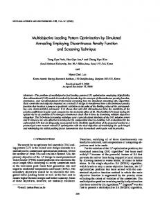
A. DTLZ 1 Figure 5 shows views in objective space of the archive obtained from a single run of each of the algorithms on test problems DTLZ1 after 5000 objective evaluations, together with plots showing the distance of the members of each set to the true Pareto front. For each algorithm, the plotted results are those which have the median distance of solutions to the true front out of a series of 20 runs; this ensures that the results presented are representative of the series. The true front for DTLZ1 is the segment of the plane passing through 0.5 on each of the objective space coordinate axes, and it can be seen that the majority of solutions generated by MOSA lie very close to the front. This test problem has a large number (≈ 115 ) of local fronts which lie as planes parallel to and further from the origin than P; the existence of these fronts is evident from the histogram of the distances from P which shows solutions clustered at two distinct distances for MOSA and several for NSGA-II (this effect is less marked on the Nam & Park front, where the solutions are distributed more evenly across many fronts which are close in objective space). It seems likely that it is these local fronts which prevent Nam & Park’s annealer and NSGA-II from converging on the true front, since in later problems without this feature the difference in performance between the three algorithms is, while still significant, much less extreme. Figure 14 provides, for each test problem, box plots comparing the average distance of the archive to the true front, the volume measure of the archive and the size of the archive (which is a fixed value for NSGAII due to the constrained nature of the algorithm). For this DTLZ1 problem, the figure clearly illustrates that MOSA has not only converged to a set very close to the true front but that the front is also well covered as shown by the volume measure results; size the MOSA archive is unconstrained in size it has been able to generate a large archive close to and covering well the true front. We observe that the annealer on this problem converges to a local front, spreads across it until a perturbation ‘breaks through’ to a front closer to P after which the annealer explores the nearer local front, adding solutions on this front to the archive and removing solutions on the previous local front as they are dominated during the exploration. Figure 6 shows the median, maximum and minimum (over 20 runs) of the distance of the current point x to the true front P versus iteration, together with the median (over 20 runs) of the median distance of members of the archive F from P on a much longer set of runs. The presence of local fronts is

10

apparent from the ‘steps’ in the median archive distance. The current solution clearly leads the archive, particularly at later iterations when the computational temperature is low and the search is effectively a greedy search. B. DTLZ 2 Figure 7 presents the archive resulting from a representative run of the algorithms on problem DTLZ2 for 1000 function evaluations and a plot of the distances from the true front, which is the eighth of a spherical shell of radius 1, centred on the origin, lying in the positive octant. As the figure shows, the archive lies close to the optimal front for each of the algorithms, with MOSA significantly closer than the other algorithms. We remark that this problem, and several others of the DTLZ suite without a plethora of local fronts, can be successfully treated with a rapid cooling schedule, as used here. Due to the ease of convergence to the true front on this problem, we anticipate that any multi-objective optimiser will be able to produce a set of solutions close to the true front although the density and coverage may vary significantly, as is the case here. Figure 14 illustrates that, while all three algorithms have converged close to the true front, MOSA is significantly closer than NSGA-II or Nam & Parks annealer. The volume measure plot shows that the archive produced by MOSA also has a greater coverage/density of solutions; even after only 1000 evaluations, the archive size plot clearly illustrates that MOSA has already converged very close to the true front and is searching across the front improving the coverage and density. While knowledge about the applicability of a short annealing schedule would not be initially available for typical realworld problems, we anticipate that, for real-world problems, the annealer would be run with a very rapid annealing schedule initially to discover if the problem were searchable in this manner. C. DTLZ 3 A striking example of the annealer’s performance is provided in Figure 8, where its evaluation on DTLZ3 is shown for 15000 function evaluations. The Pareto front here is again an eighth of a spherical shell, preceded by multiple local fronts, of the same order as DTLZ1. The computational archive is converged to within 0.01 of the true front, as supported by the histogram of solution distances from the front in Figure 8. Consistent with the findings by Deb et al. [30] NSGAII had failed to converge (Deb et al. comment that in their experiments that NSGA-II had still failed to converge after 50000 function evaluations) and Nam and Park’s annealer yields performance similar to NSGA-II (as illustrated in Figure 14). Consistent with the previous problems, MOSA’s archive is shown to be large, dense and well covering in Figure 14. D. DTLZ 4 The true Pareto front for this problem is again an eighth of a spherical shell, but the solutions are unevenly distributed


MOSA − DTLZ2

UNDER REVIEW

11

Nam & Park − DTLZ2

1.5

NSGA−II − DTLZ2

1.5

1.5

1

1

1

0.5

0.5

0.5

0 0

0 0

1 0.5

0.5

1.5 0.5

1

0.5

1

0 0

1.5 1

1.5 0

1 1

0.5 1.5 0

0.5 1.5 0

6

4 140

3.5 120

5

3

4

100

2.5

80

2

3

60

1.5

2

40

1

20

0.5

0 0

0.005 0.01 Distance from the true Pareto front

1

0 0

0.015

0.1 0.2 0.3 0.4 Distance from the true Pareto front

0 0

0.05 0.1 0.15 0.2 0.25 0.3 Distance from the true Pareto front

Fig. 7. Top: Archives on test problem DTLZ2 after 1000 function evaluations. Bottom: Histograms of archive member distances from the true Pareto front (the 5% most distant have been omitted to aid visualisation). MOSA − DTLZ3 Nam & Park − DTLZ3

1.5 1 0.5 0 0

1500

1500

1000

1000

500

500

0 0

1.5 0.5

1 1

NSGA−II − DTLZ3

1500 500

500

500

0.5 1.5 0

0 0

1000

1000 1000

1000 0

500 1500 0

7

400

5

350

6

300

5

250

4

200

4

3

3 2

150

2 100

0 0

1

1

50 0.02 0.04 0.06 Distance from the true Pareto front

0 0

200 400 600 800 1000 Distance from the true Pareto front

0 0


1200

Fig. 8. Top: Archives on test problem DTLZ3 after 15000 function evaluations. Bottom: Histograms of the distance from the true Pareto front of the archive members (the 5% most distant have been omitted to aid visualisation).

across it. Figure 9 shows the algorithms’ archives after 5000 function evaluations, showing that solutions are concentrated close to the f1 − f3 and f1 − f2 planes together with a less dense covering of the shell between them for MOSA and Nam & Park’s algorithm, while NSGA-II achieves an even

coverage. Though the distribution of points across the front is more even with NSGA-II than MOSA, MOSA produced solutions which were far closer to the true front. Figure 14 shows that the solutions generated by MOSA have a much lower volume measure; although visually the solutions from


UNDER REVIEW

12


MOSA − DTLZ4

NSGA−II − DTLZ4

1

2

0.5

1

0 0

0 0

1.5 1 0.5

0.5

1

1

3

6

100

2.5

5

80

2

4

60

1.5

3

40

1

2

20

0.5

1

0 0

0.5 1.5 0

120

1 2 3 4 Distance from the true Pareto front x 10−4

1

2 0

1.5 0

0 0

1.5 0.5

1

0.5

1

0 0

2

1


0 0


0.4


the NSGA-II runs seem superior to MOSA’s, the performance metrics suggest that MOSA has produced a better estimation of the true front. Deb et al. [26] observe that each run of NSGA-II in their experiments converged to a different part of the Pareto front; either to the f1 -f2 plane, the f3 -f1 plane, or distributed across the curved region of the front between these planes. The reason for the improved coverage of the PISA NSGA-II implementation is that the clustering close to the rims characteristic of the problem increases as solutions approach the true front. It is much more likely for solutions situated increasingly far from the true Pareto front to lie behind the central region of the front, although also to be dominated by the rims. E. Density of solutions on the front MOSA solutions on the front located by the annealer for problem DTLZ4 are close to the true Pareto front, but they are clearly inhomogeneously distributed across the front. Likewise, it is apparent from Figures 5, 7 and 8, for problems DTLZ1, DTLZ2 and DTLZ3, that the density of solutions is greater close to the f1 − f2 plane than distant from it. Here we discuss in some detail the reasons for this inhomogeneity. As we alluded to in section III, when x and x0 both lie on or very close to P then δE(x0 , x) = 0 and all proposals lying on the front are accepted, so that the trajectory of the current solution is a random walk in parameter space. The density of solutions on this front in objective space is governed by the mapping of area or volume from parameter space to objective space. Assuming that the fi (x) are continuous in a neighbourhood of x, the mapping is locally linear and

is described by the D by N Jacobian matrix of partial derivatives:3 Jij (x) =

∂fi (x). ∂xj

(16)

It is useful to write J in terms of its singular value decomposition (SVD; see, for example, [34]): J = UΣVT

(17)

Here U is a D by D matrix whose orthonormal columns ui (i = 1, . . . , D) form a local basis for objective space at f (x). Likewise, the D columns of V ∈ RN ×D , denoted vi , (i = 1, . . . , D) are orthonormal N -dimensional vectors forming a local basis for the D-dimensional subspace of parameter space that locally maps to objective space. The matrix Σ ∈ RD×D is diagonal, whose diagonal elements σi ≥ 0 are known as singular values and are conventionally listed in descending order so that σ1 ≥ σ2 ≥ . . . σD ≥ 0. The singular value σi quantifies the magnification of a perturbation in direction vi in parameter space: thus a small perturbation about x of vi in parameter space yields a change in objective space from f (x) to f (x) + σi ui . If x lies on the Pareto front no parameter space perturbation can result in a change in objectives normal to the front, implying that one of the singular values is zero and the rank of J is at most (D − 1). Assuming for simplicity that the Pareto front is (D − 1)-dimensional, the direction normal to the front corresponds to uD and vD in objective and parameter spaces 3 In real problems the Jacobian matrix may be estimated by finite differences or computer-aided differentiation packages, e.g. [33]


UNDER REVIEW

13

0.7

0.6 2

0.5

1.5 0.5

1

0.4

0.4

0.8

0.3

0

0.6

0.3

0.2

0

0.4 0.1

0.1

0.2

0

0

0.2

0 0.1

0.5 0.2

0.6

0.1

0.2 0.3

0.4

0

0.3

1

0.2

0.2

0.4 0.6

0.4 0.4

0.8 0.8

0.5

0.5

1

1

5 90 4.5 80 4 70 3.5 60 3 1

1 50

0.8

0.8

2.5

0.6

0

0.4

0.6 2

0.2

0.2

0 0.2

0.2

30

1.5 0

0

0.4

0

0.4

0

1 0.2

20 0.2

0.6 0.4

0.6 0.4

0.5 0.6

40

0.4

10 0.6

0.8 0.8

0.8 0.8

1

1

1

1

Fig. 10. Magnification factors on the Pareto front. Top left: DTLZ1; Top right: DTLZ3; Bottom left: DTLZ4 with α = 2; Bottom right: DTLZ4 with α = 10. Colour indicates the local volume magnification factor from parameter space to objective space. Nam & Park − DTLZ5

MOSA − DTLZ5

1.5

NSGA−II − DTLZ5

2

2

1

1

1 0.5 0 0

1

0 0

1.5 0.5

0.5

0.5

0 0

1

1 1

0.5 1.5 0

1 0

1.5 0.5

1

0.5 1.5 0

7

6

6

5

18 16

5

14 12

4

4

10

3

8

3

6

2

2

4

0 0

1

1

2 0.002 0.004 0.006 0.008 0.01 0.012 0.014 Distance from the true Pareto front

0 0


0.8

0 0

0.1 0.2 0.3 0.4 0.5 0.6 Distance from the true Pareto front



UNDER REVIEW

respectively, and σD = 0. Perturbations lying in the span of v1 , . . . , vD−1 result in traversal movements along the front and the (infinitesimal) volume in parameter space νp lying in span(v1 , . . . , vD−1 ) is magnified to volume νo = ν p

D−1 Y

σi .

(18)

i=1

on the Pareto front. These ideas are illustrated in Figure 10, which shows the volume magnification factor on the front for DTLZ1, DTLZ3 and DTLZ4. These were calculated by evaluating the Jacobian matrix at a large number of points in parameter space using a symbolic algebra package and then numerically finding the singular values. Comparison with Figures 5 and 8 for DTLZ1 and DTLZ3 makes it apparent that the magnification factors correspond to the density of solutions generated by the simulated annealer. If XP = f −1 (P) is the (D − 1)dimensional manifold in parameter space that maps to the Pareto front, then this may be understood in terms of the annealer performing a random walk on XP which it covers fairly uniformly, producing a high density of solutions in objective space where the magnification factor is low, but a low density of solutions where the magnification factor is high because here solutions in parameter space are spread more thinly in objective space. The bottom panels of Figure 10 show the local volume magnification factors for DTLZ4, but with α = 2 and α = 10, rather than α = 100 as recommended by Deb et al. [26], [30]. As the figure indicates, the magnification factor at points on the front even for α = 10 is almost two orders of magnitude greater than the magnification factors for DTLZ1 and DTLZ3; when α = 100 the pattern of magnification factors is similar but the range of magnifications is too great for sensible visualisation. The magnification is least close to the f1 − f2 and f1 − f3 planes, corresponding precisely to the regions in which plenty of solutions are located by the annealer (Figure 9) and greatest on the section of the front close to the f2 − f3 plane where few solutions are located. We infer that the annealer is locating and exploring XP in this case, but we see few solutions on parts of the front because the magnification factors are extremely high. These deliberations lead us to consider again the question of what is an appropriate natural measure on the Pareto front. In our formulation of a multi-objective simulated annealer we used an approximation to the Lebesgue measure, namely the number of solutions in the archive, to evaluate the energy of a solution (9). However, this measure is defined in objective space and it might be argued that a more natural measure in objective space is the one induced by Lebesgue measure on XP . In fact, as our experiments show, once the vicinity of the Pareto front has been located it is (approximately) this induced measure that governs the density of solutions located. One may envisage that the singular value decomposition of J may be used to counteract the inhomogeneity produced in objective space by the magnification factor by biasing the perturbations along the singular vectors vi associated with large singular values σi . This is the subject of current research.

14

F. DTLZ 5 Figure 11 shows the archives generated by the algorithms after 1000 function evaluations on test problem DTLZ5 for which the front is a one-dimensional curve rather than a full two-dimensional surface. As the distance plots show, the annealer has successfully located the one-dimensional front while the other two algorithms generate sets which reside some distance behind this front; Deb et al. [26] also report that NSGA-II had not fully located the curve and yields a surface a little above the curve even after 20000 function evaluations in their experiments. Figure 14 shows that the MOSA archive almost completely dominates the space dominated by the true front; the true front is almost completely covered by the archive. This is the only test problem in which MOSA’s archive does not grow larger (in the allowed iteration count) than NSGA-II’s (enforced) set of 100 results, this is not especially significant however, as the NSGA-II set is significantly less well converged than MOSA’s archive. G. DTLZ 6 The front for DTLZ6 consists of four disjoint components.4 As Figure 12 shows the annealer is able to successfully locate each of these components during a single run, that NSGA-II is able to generate solutions close to each front and that Nam & Park’s annealer does not converge in the allowed number of evaluations. Figure 14 shows that, again, MOSA’s coverage of the front, as well as the distance from the true front, dominates almost all the feasible search space. During optimisation (and once the archive is close to the true Pareto front) we observe that the current solution x of MOSA explores one component of the front for a few proposals before ‘jumping’ to another component. If the regions of parameter space corresponding to each of the components of the front were widely separated then it might be considerably more difficult for the annealer to simultaneously locate all components. H. DTLZ 7 The DTLZ7 test problem is constructed using multiple constraint surfaces to yield a Pareto front consisting of a triangular planar section and a line segment. Figure 13 shows the algorithm archives after 9000 function evaluations. The particular way in which DTLZ7 is constructed means that a perturbation of a single parameter of a solution lying on the front makes the perturbed parameter vector infeasible because it violates one of the constraints. Our schemes, described in section V-B, for adjusting the perturbation scalings rely on perturbing a single parameter at a time in order to keep track of the effect of the perturbation. However, this renders them ineffective for this problem: a single solution on the front is rapidly located, but the annealer is unable to explore the front because all perturbations result in infeasible proposals. For this reason the archive shown in Figure 13 was generated by perturbing a randomly chosen number of parameters for each 4 We use the formula given in [26], [30]; the figures in these publications appear to have been generated with the f3 objective scaled by a factor of 2.


MOSA − DTLZ6

UNDER REVIEW

15


NSGA−II − DTLZ6

8

18

15

6

16

10

4

14

5

2 0

1 0.5

12 0

0 0

1 0.5

0.5

1 0.5

0.5

1 0

0.5

1 0

12

1 0

14

2

12

10 1.5

10

8

8 6

1

6

4

4

0.5

2

2

0 0

0 0

0.05 0.1 Distance from the true Pareto front


0 0

12

1 2 3 4 Distance from the true Pareto front

Fig. 12. Top: Archives on test problem DTLZ6 after 5000 function evaluations for each of the three algorithms. Bottom: Histograms of the distance from the true Pareto front of the archive members (the 5% most distant have been omitted in each of the 6 figures to aid visualisation). Nam & Park − DTLZ7

MOSA − DTLZ7

NSGA−II − DTLZ7

1

20

1

0.5

15

0.5

0 0

1 0.5

10 0

0 0

1 0.5

0.5

1 0.5

0.5

0.5

1 0

1 0

1 0 8

3

120

7 2.5

100

6 80

2

60

1.5

40

1

20

0.5

5

4

3

2

1

0 0

0.02

0.04


0.14

0.16

0.18

0 11

12

13

14 15 16 Distance from the true Pareto front

17

18

0 0

0.05

0.1


0.3

0.35

Fig. 13. Left: Archives on test problem DTLZ7 after 9000 function evaluations for each of the three algorithms. Right: Histograms of the distance from the true Pareto front of the archive members (the 5% most distant have been omitted to aid visualisation in all 6 figures).

proposal; for simplicity the perturbation scales were kept constant at 0.1 of the feasible region throughout the optimisation. While more efficient perturbation schemes could probably be devised, the figure shows that the annealer is reasonably successful in locating the central portion of the front, although

the extremities of the front have not been explored and there remain some extraneous solutions close to constraint surfaces bounding the front, but still quite distant from P itself. We also modified the single parameter perturbation scheme used in our implementation of Nam & Park’s annealer to perform


UNDER REVIEW

the same multiple point perturbations as MOSA. NSGA-II, the PISA implementation of which already used a (more advanced) multiple parameter perturbation, did not need to be modified for this problem. Figures 13 and 14 show that, while MOSA has again converged well, and generates the solutions closest to, the true front, NSGA-II demonstrates the best coverage of solutions over the front towards the extremes of the constraints. It should be noted that the need to adapt to a multiple parameter perturbation scheme will be present for all algorithms which employ a specialised single parameter perturbation scheme (conversely, problems can be constructed that would prevent a multiple parameter perturbation scheme from converging to the true front). I. Statistical performance measures Unlike single objective problems, solutions to multiobjective optimisation problems can be assessed in several different ways. Therefore in order to quantify the convergence of the algorithms we measure two distinct properties. Firstly, we calculate the average distance of the archived solutions discovered from the true front to ascertain how close on average solutions found are to the true front. Rather than using the root mean square distance which is susceptible to outliers, here we use the median distance of solutions in the archive: ¯ ) = median[d(x)] d(F

(19)

x∈F

where d(x) is the minimum Euclidean distance between x and the true front P. Clearly, this measure depends on the relative scaling of the objective functions, however, it yields a fair comparison here because the objectives for the DTLZ test functions have similar ranges. Secondly, since we are concerned with finding solutions spread across the true Pareto front, we also use a variant of the volume V measure [22] which is conceptually similar to the performance measure used in [35]. The idea is to calculate the amount of objective space that is dominated by the true front, but not by the calculated archive. To make this precise, let H be the minimum axis-parallel hypercube in objective space which contains P. Then V(P, F ) is the fraction of H which is dominated by P but not by F . Clearly this measure is zero when F covers the entire Pareto front and it approaches zero as F approaches P . Importantly however, an archive comprised of a few solutions clustered together on the true front will have a larger V(P, F ) than an archive of solutions well spread across the front and therefore dominating a larger fraction of objective space. This measure is straightforwardly calculated by Monte Carlo sampling (105 samples here) of H and counting the fraction of samples dominated exclusively by P and not F ; see [22] for details. Figure 14 shows box plots over 20 runs, from different randomly-selected initial solutions, of the median Euclidean ¯ ), fractional volume measures and archive size distance, d(F of the results for each algorithm on each test problem. The distance of P to the objective space origin is O(1) for all of these problems, so it can be seen from Figure 14 that the annealer is able to converge very close to the front for

16

all seven problems. In fact, MOSA is significantly closer to the front, (as described in section VI) than both NSGA-II and Nam & Park’s annealer. NSGA-II was able to converge to a set near to the true front for five of the problems (with two of those being very near) and Nam & Park’s annealer was able to generate an archive near the true front on one of the problems. The middle row of Figure 14 shows V(P, F ), the fractional volume dominated by P and not by F . As the figure indicates the annealer both converges well to P and also covers it reasonably well for all the problems. MOSA dominates significantly more volume than NSGA-II for 6 of the 7 cases although NSGA-II is significantly better on DTLZ7. NSGA-II achieved a good coverage on those problems for which it could converge near to the true front; the diversity maintainance in the algorithm encourages this. NSGA-II performed particularly well on DTLZ7 where the coverage was better than MOSA’s. Nam & Park’s algorithm was unable to effectively cover the true front for any problem. The results for DTLZ4 effectively demonstrate why it is necessary to measure convergence in terms of both distance and coverage, with MOSA having converged close to P, but yielding a poor coverage of the front (in objective space), an artifact of the large range of volume magnification factors, as discussed earlier, also demonstrating that the visually appealing NSGA-II results were less well converged than it seems upon inspection. Confirming the impression given by the single run depicted in Figure 13, on average the annealer does not completely cover the true front for DTLZ7. As discussed above this could probably be improved by designing particular perturbation strategies for this particular problem; the NSGA-II implementation has a multiple point mutation scheme which performs very well on this problem. Figure 14 also shows how the final archive size varies across the 20 runs for each of the DTLZ problems used here. For the MOSA results it is clear that even the fronts generated by the least well-covered runs for each problem contain a large quantity of solutions relative to the run length. Furthermore the number of solutions generated for each problem is consistent across runs, although, as may be expected, problems with multiple local fronts (DLTZ1 and DTLZ3) have a larger spread. The NSGA-II algorithm is constrained to a predefined size (100 solutions in the work presented here) and Nam & Park’s annealer does not generate large sets of solutions as it does not converge close to the true front. VII. CDMA

NETWORK OPTIMIZATION

Mobile telephone subscribers are allocated to one of a number of distinct cells or sectors comprising the telephone network. Cells may vary in extent from a few tens of metres (in a large office building) to several kilometres (in rural areas). Each cell is served by a single antenna and as the phone subscriber moves to a new location a ‘handover’ is made to a new cell in which the radio signal is stronger. The performance of the network whole and the quality of service enjoyed by individual subscribers is dependent upon a great many operating parameters, some associated with the antenna and radio interface itself (such as the antenna azimuth and


DTLZ1

DTLZ2

UNDER REVIEW

DTLZ3

DTLZ4

700

DTLZ6

10

0.6

0.45

14

0.25 80

0.4

500

0.5

12

8

0.35

0.2 400

60

6 8

0.25

300

10

0.4

0.3

0.15

0.3

0.2

40 0.1

200

6

4 0.2

0.15

4 20

0.1

0.05

100

0

0

2

0.1

2

0.05 0 MOSA NSGAII N&P

MOSA NSGAII N&P

DTLZ1

Volume measure

0.8

0 MOSA NSGAII N&P

DTLZ3 1

0.8

0.9

0 MOSA NSGAII N&P

DTLZ2 0.9

1

0.7

0.9 0.9 0.8 0.8 0.7

0.6 0.5

0.4

0.6 0.5 0.4

0.4 0.3

0.2

0.2

0.3

0.1

0.3 0.3

0.4 0.2

0.2 0.2

0.1

0.1

0.1

0.1

0

0.1

DTLZ1

0.7

0.5

0.5

0.3

MOSA NSGAII N&P

0.8

0.5

0.3

0.2

0.9

0.8

0.4

0.4

0.4

0.9

0.6

0.6

MOSA NSGAII N&P

MOSA NSGAII N&P

DTLZ2

DTLZ3

MOSA NSGAII N&P

DTLZ4

MOSA NSGAII N&P

MOSA NSGAII N&P

DTLZ5

DTLZ6

400

300

DTLZ7

110

2500

900

350

400

100

200

250 2000

300

90

250

80

800 700

300

150

200 1500

250

MOSA NSGAII N&P

1000

450

350

DTLZ7 1

0.6

0.5

0.5

DTLZ6

0.7

0.6

MOSA NSGAII N&P

1

0.7

0.7

0.6

MOSA NSGAII N&P

DTLZ5 1

0.8

0

0 MOSA NSGAII N&P

DTLZ4 1

0.9

0.7

0.3

Archive size

DTLZ7 16

0.5 600

Euclidean distance from true front

DTLZ5 0.7

0.3

100

17

600

70 200

500 60

200 150

1000

400

100

150

50

150

300 40

100 100

500

100

100 20

0

0 MOSA NSGAII N&P

MOSA NSGAII N&P

200

50

30

50

50

MOSA NSGAII N&P

MOSA NSGAII N&P

MOSA NSGAII N&P

MOSA NSGAII N&P

0

MOSA NSGAII N&P

¯ ) of the archive from the true Pareto front for 20 runs of each DTLZ test problems, using the documented Fig. 14. Top: Box plots of the average distance d(F run lengths. Middle: Box plots of the volume measure V(P, F ) of the archive for each run. Bottom: Box plots of the size of the archive for each run. Each figure shows the results for MOSA, NSGA-II and Nam & Park’s annealer.

downtilt) and others associated with the network as a whole, such as the handover policy [36]. In addition performance itself may be evaluated in terms of several different metrics, for example: the network capacity (number of simultaneous calls); coverage (area served); and mean cell traffic channel power. The simultaneous optimisation of all these competing objectives is generally impossible and here we use the MOSA to investigate the trade-offs between them. We draw attention to recent work using multi-objective optimisation in the mobile telecommunications domain: Ben Jamaa et al. [37] have used multi-objective genetic algorithms for cell planning in order to optimise the cost and coverage of a network, and Szabó et al. [38] have used multi-objective evolutionary algorithms for discovering the cost-interference trade-off when allocating transmitter placement and assigning transmission frequencies in time division multiple access (TDMA) networks.

We treat as parameters to be optimised the pilot powers of a CDMA network. The pilot power may be loosely thought of as the power with which the cell transmits to establish initial communication with phones in its cell. Pilot power is a particularly important parameter in CDMA (Code Division Multiple Access) networks because cells transmit continuously and if the pilot power is too great a cell may drown out its neighbours, but will not be heard if the pilot power is too low. In this study there were 94 pilot powers as parameters and we optimised three objectives: the pilot pollution factor, defined as the number of pilots that each subscriber receives within 5dB of the dominant pilot; the mean downlink traffic channel (TCH) outage factor defined as the number of subscribers attempting to exceed their TCH power limit; and the mean reverse link server penalty which quantifies the unbalancing of the reverse link. This is done by comparing the propagation


UNDER REVIEW

18 Network 1 (low TCH outage)

Network 2 (high pilot pollution)

0.16

Reverse link server penalty

0.14 0.12 0.1

Network 3

0.08 0.06 0.04

Network 4 Network 1

0.02 0 4

Network 3

5

Fig. 15.

Network 4

Network 2

4.5

TCH Outage %

(high reverse link penalty)

1.54

1.56

1.58

1.6

1.62

1.64

1.66

1.68

Pilot Pollution Factor

Estimated Pareto front for network pilot power optimisation.

loss between each subscriber and its serving cell and the smallest propagation loss between that subscriber and any cell—the average difference between these values across all subscribers is defined as the reverse link penalty. Unlike optimisation of test problems, as in section VI, the properties of the CDMA search space are not known in advance. Particularly, it is not known if the problem exhibits local front behaviour, where an optimiser must make several successive movements out of a locally optimal region of parameter space in order to locate the globally optimal region which corresponds to the Pareto front in objective space. The results reported here are for an operational CDMA-1X network consisting of 94 sectors. Computational optimisation is feasible for this system due to the employment of a proprietary mathematical model of the downlink air interface which permits rapid evaluation of new configurations. In this study the pilot power of each sector was allowed to vary over the range from 1.0W to 3W in 0.5W intervals. Initially the pilot powers were set to their minimum feasible values and the MOSA was initialised to a temperature that yielded a 50% acceptance rate for derogatory moves, as described in section V-A. The computational temperature was then reduced every Lk = 100 proposals by a factor of βk = 0.958. The annealer was run for 100000 evaluations of the objective function. Figure 15 shows the estimated Pareto front obtained, which consists of 965 solutions. We remark that a standard genetic algorithm optimising a composite objective function locates after 100000 function evaluations a single solution which is dominated by almost all of the non-dominated archive. The GA solution is distant from the archive but it is likely that the genetic algorithm would have located a point in the vicinity of the front generated by the simulated annealer if it had been permitted a greater number of objective evaluations. Of course the principal advantage of the annealer is not the reduction in the time taken to find a desirable solution (although this is considerable), but the frontal nature of the results generated by the simulated annealer. The front which has been located is clearly curved in objective space and displays to the network engineer the range of trade-offs which may be made in configuring the network.

Fig. 16. Pareto-optimal central network configurations corresponding to the labelled points on the Pareto front in Figure 15.

The central portion of the network configuration corresponding to each of the solutions circled in Figure 15 is shown in Figure 16. In this figure, the pilot power for a sector is indicated by the length of an arrow rooted at the antenna location (antennae masts frequently support two or three antennae serving different sectors). It is interesting to note that each of the network configurations is very similar, despite their extreme relative frontal locations. This figure provides important information about the network to a network engineer, since some pilot powers seem to have single optimal values, particularly those in the less populated areas of the network with fewer interactions. However, as might be expected, it can be seen that the configuration with low pilot pollution (network 3) restricts pilot powers in sectors that face each other. The interaction between pilot powers and the other objectives is less clear, but the MOSA methodology provides a mechanism for locating these optimal configurations. Current work involves applying this methodology to the optimisation of antennae pilot powers, azimuths and downtilts in larger networks. VIII. C ONCLUSIONS We have presented an energy measure for use in multiobjective SA which is based on the fundamental notion of dominance, rather than employing a weighted combination of the objectives. Simulated annealers employing this measure were shown to have good convergence properties on the first seven DTLZ test functions [26], [30]. An extensive comparison with the evolutionary algorithm NSGA-II and the multi-objective annealer proposed by Nam & Park [8] on these problems shows that the annealer consistently generates archives closer to the true front than NSGA-II and Nam & Park’s annealer and that in all but one case produces a significantly better coverage (on DTLZ7 NSGA-II generates fronts with a fuller coverage of the front, possibly due to the more specialised multiple point perturbations used).


UNDER REVIEW

We emphasise that MOSA the algorithm was not ‘tuned’ for each of these problems, but run from a randomly chosen initial condition. More rapid convergence on many of these problems can be achieved by careful tuning of the annealing schedule but, of course, this requires many runs to discover a reasonable schedule; while tuning the annealing schedule is important in industrial applications where the annealer is to be run many times on similar problems (e.g., CDMA network optimisation), we have refrained from tuning the annealer to particular test problems; here we simply limit all the algorithms to an evaluation count approximately at which the first algorithm converges on the true front. The only instance in which it was necessary to alter the annealers was for DTLZ7, for which single point perturbations of solutions close to the Pareto front result in infeasible proposals, however, it should be noted that the problem with single point perturbations will afflict all stochastic searches (evolutionary algorithms, GAs, etc) that perturb a solution to generate a new candidate solution and that in this problem, MOSA performed almost as well with a very basic multiple point perturbation scheme as NSGA-II did, which uses a more advanced scheme. An advantage of the dominance based energy measure is that it is not a priori biased towards any part of the front. Weighted sum optimisers implicitly use distance information in objective space, which renders them sensitive to the relative scalings of the objectives, whereas our algorithm is robust to rescalings of the objectives. Indeed, if the relative importance or scales of the objectives were known in advance it might be more straightforward to optimise a single, appropriately weighted, sum of the objectives. Notions of dominance and Pareto optimality are well suited to handling competing objectives whose relative importance is a priori unknown and it is therefore natural to eschew metric information in favour of dominance concepts in order to guide the search. Indeed, we have argued that the dominance based energy tends to promote exploration in sparsely populated regions and in practice we have shown that estimated fronts evenly and widely cover the true front. An area of current investigation is to use the singular values and vectors of the Jacobian matrix to guide the search on the front towards areas that would be otherwise be sparsely populated. Determining an efficient scale on which to make proposals is more complicated in the multi-objective case than the uniobjective case, because some proposals work to advance the front, while others traverse the front. We have proposed simple heuristics to adapt the perturbation scales and future work involves applying machine learning techniques to learn the local mapping between parameter and objective space in order to more sensitively control the search direction. When applied to the optimisation of a CDMA network the annealer is successful in generating a front with a large number of mutually non-dominating solutions, the vast majority of which are superior to the single solution located by a genetic algorithm optimising a composite objective function. This allows a network engineer to make an informed decision regarding network configurations with additional knowledge of the costs of the trade-offs involved. Further work in this direction involves the optimisations involving both more

19

parameters, such as antenna azimuths and downtilts, and additional objectives relating to the quality of service for subscribers. Our E(x) is a measure of a portion of the dominating set, namely µ(F˜x ), which is a close relation to Fleischer’s recently proposed measure [20]; loosely, our measure deals with the area of the dominating surface—the attainment surface— while Fleischer’s considers the dominated volume. It would be interesting to investigate the convergence of an annealer based on Fleischer’s measure but, as shown in [39], the complexity of the calculation is polynomial in the number of archived solutions and exponential in the number of objectives; this makes calculation for even 3 objectives infeasibly slow for use as the energy calculation for an annealer. Although a proof of convergence for simulated annealers based on our measure remains to be completed, this is an area of current work, together with the application of the annealer to other large scale problems. Acknowledgements The authors would like to thank Michelle Fisher and the anonymous reviewers for their useful comments. We would also like to thank the authors of the PISA code [32] for making their implementation of the NSGA-II algorithm available for use by the academic community. R EFERENCES [1] S. Kirkpatrick, C. Gelatt, and M. Vecchi, “Optimization by simulated annealing,” Science, vol. 220, pp. 671–680, 1983. [2] N. Metropolis, A. Rosenbluth, M. Rosenbluth, A. H. Teller, and E. Teller, “Equation of state calculations by fast computing machines,” Journal of Chemical Physics, vol. 21, pp. 1087–1092, 1953. [3] S. Geman and D. Geman, “Stochastic relaxation, Gibbs distributions, and the Bayesian restoration of images,” IEEE Transactions on Pattern Analysis and Machine Intelligence, vol. 6, pp. 721–741, 1984. [4] C. Coello, “A Comprehensive Survey of Evolutionary-Based Multiobjective Optimization Techniques,” Knowledge and Information Systems. An International Journal, vol. 1, no. 3, pp. 269–308, 1999. [Online]. Available: citeseer.nj.nec.com/coello98comprehensive.html [5] D. V. Veldhuizen and G. Lamont, “Multiobjective Evolutionary Algorithms: Analyzing the State-of-the-Art,” Evolutionary Computation, vol. 8, no. 2, pp. 125–147, 2000. [6] P. Engrand, “A multi-objective approach based on simulated annealing and its application to nuclear fuel management,” in 5th International Conference on Nuclear Engineering, Nice, France, 1997, pp. 416–423. [7] P. Czy˙zak and A. Jaszkiewicz, “Pareto simulated annealing – a metaheuristic technique for multiple-objective combinatorial optimization,” Journal of Multi-Criteria Decision Analysis, vol. 7, pp. 34–47, 1998. [8] D. Nam and C. Park, “Multiobjective simulated annealing: a comparative study to evolutionary algorithms,” Internation Journal of Fuzzy Systems, vol. 2, no. 2, pp. 87–97, 2000. [9] M. Hapke, A. Jaszkiewicz, and R. Slowinski, “Pareto simulated annealing for fuzzy multi-objective combinatorial optimization,” Journal of Heuristics, vol. 6, no. 3, pp. 329–345, 2000. [10] A. Suppapitnarm, K. Seffen, G. Parks, and P. Clarkson, “A simulated annealing algorithm for multiobjective optimization,” Engineering Optimization, vol. 33, pp. 59–85, 2000. [11] K. Smith, R. Everson, and J. Fieldsend, “Dominance measures for multi-objective simulated annealing,” in Proceedings of Congress on Evolutionary Computation, CEC04, 2004, pp. 23–30. [12] L. Ingber, “Simulated annealing: Practive versus theory,” Mathematical Computation and Modelling, vol. 18, pp. 29–57, 1993. [13] P. Salamon, P. Sibani, and R. Frost, Facts, Conjectures, and Improvements for Simulated Annealing, ser. Monographs on Mathematical Modeling and Computation. Society for Industrial and Applied Mathematics, 2002, no. 7.


UNDER REVIEW

[14] P. Serafini, “Simulated annealing for multiobjective optimization problems.” in Multiple criteria decision making. Expand and enrich the domains of thinking and application, 1994, pp. 283–292. [15] E. Ulungu, J. Teghaem, P. Fortemps, and D. Tuyttens, “MOSA method: a tool for solving multiobjective combinatorial decision problems,” Journal of multi-criteria decision analysis, vol. 8, pp. 221–236, 1999. [16] D. Tuyttens, J. Teghem, and N. El-Sherbeny, “A particular multiobjective vehicle routing problem solved by simulated annealing,” in Metaheuristics for multiobjective optimisation, ser. Lecture notes in economics and mathematical systems, X. Gandibleux, M. Sevaux, K. Sörensen, and V. T’kindt, Eds. Springer, 2003, vol. 535, pp. 133–152. [17] M. Hapke, A. Jaszkiewicz, and R. Slowinski, “Pareto simulated annealing for fuzzy multi-objective combinatorial optimization,” Journal of heuristics, vol. 6, no. 3, pp. 329–345, 2000. [18] I. Das and J. Dennis, “A closer look at drawbacks of minimizing weighted sums of objectives for pareto set generation in multicriteria optimization problems,” Structural Optimization, vol. 14, no. 1, pp. 63– 69, 1997. [19] A. Jaszkiewicz, “Comparison of local search-based metaheuristics on the multiple objective knapsack problem,” Foundations of computer and decision sciences, vol. 26, no. 1, pp. 99–120, 2001. [20] M. Fleischer, “The measure of Pareto optima: Applications to multiobjective metaheuristics,” in Evolutionary Multi-Criterion Optimization, Second International Conference, EMO2003, ser. Lecture Notes in Computer Science, C. Fonesca, Ed., vol. 2632. Springer, 2003, pp. 519–533. [Online]. Available: http://link.springer.de/link/service/series/ 0558/bibs/2632/26320267.htm [21] D. Greening, “Simulated annealing with inaccurate costs functions,” in Proceedings of the IMACS International Congress of Mathematics and Computer Science, Trinity College, Dublin, 1993. [Online]. Available: citeseer.nj.nec.com/article/greening94simulated.html [22] J. Fieldsend, R. Everson, and S. Singh, “Using Unconstrained Elite Archives for Multi-Objective Optimisation,” IEEE Transactions on Evolutionary Computation, vol. 7, no. 3, pp. 305–323, 2003. [23] M. T. Jensen, “Reducing the Run-time Complexity of Multi-Objective EAs: The NSGA-II and other Algorithms,” IEEE Transactions on Evolutionary Computation, vol. 7, no. 5, pp. 502–515, 2003. [24] E. Zitzler, “Evolutionary Algorithms for Multiobjective Optimization: Methods and Applications,” Ph.D. dissertation, Swiss Federal Institute of Technology Zurich (ETH), 1999, diss ETH No. 13398. [25] V. G. da Fonseca, C. Fonseca, and A. Hall, “Inferential Performance Assessment of Stochastic Optimisers and the Attainment Function,” in First International Conference on Evolutionary Multi-Criterion Optimization, E. Zitzler, K. Deb, L. Thiele, C. Coello, and D. Corne, Eds. Springer-Verlag. Lecture Notes in Computer Science No. 1993, 2001, pp. 213–225. [Online]. Available: citeseer.nj.nec.com/590159.html [26] K. Deb, L. Thiele, M. Laumanns, and E. Zitzler, “Scalable multiobjective optimization test problems,” in Congress on Evolutionary Computation (CEC’2002), vol. 1, 2002, pp. 825–830. [27] M. Laumanns, G. Rudolph, and H. Schwefel, “Mutation control and convergence in evolutionary multi-objective optimisation,” in Proceedings of the 7th International Mendel Conference on Soft Computing (MENDEL 2001), R. Matousek and P. Osmera, Eds., Brno, Czech Republic, 2001, pp. 24–29. [28] I. Sbalzarini, S. Müller, and P. Koumoutsakos, “Microchannel optimization using multiobjective evolution strategies,” in Proceedings of the First International Conference on Evolutionary Multi-Criterion Optimization (EMO), ser. Lecture Notes in Computer Science, E. Zitzler, K. Deb, L. Thiele, C. Coello Coello, and D. Corne, Eds. Springer, 2001, pp. 516–530. [29] D. Büche, S. Müller, and P. Koumoutsakos, “Self-adaptation for multiobjective evolutionary algorithms,” in Evolutionary Multi-Criterion Optimization, Second International Conference, EMO 2003, Faro, Portugal., ser. Lecture Notes in Computer Science, C. Fonseca, P. Fleming, E.Zitzler, K. Deb, and L. Thiele, Eds., vol. 2632. Springer, 2003, pp. 267–281. [Online]. Available: http://link.springer.de/link/ service/series/0558/bibs/2632/26320267.htm [30] K. Deb, L. Thiele, M. Laumanns, and E. Zitzler, “Scalable multiobjective optimization test problems,” Institute für Technische Informatik und Kommunikationsnetze, ETH Zurich, Tech. Rep. 112, 2001. [31] K. Deb, S. Agrawal, A. Pratap, and T. Meyarivan, “A Fast Elitist NonDominated Sorting Genetic Algorithm for Multi-Objective Optimization: NSGA-II,” in Proceedings of Parallel Problem Solving from Nature PPSN VI. Springer, 2000, pp. 849–858. [32] S. Bleuler, M. Laumanns, L. Thiele, and E. Zitzler, “PISA — a platform and programming language independent interface for search algorithms,” in Evolutionary Multi-Criterion Optimization (EMO 2003), ser. Lecture

[33] [34] [35] [36] [37] [38]

[39]

20

Notes in Computer Science, C. M. Fonseca, P. J. Fleming, E. Zitzler, K. Deb, and L. Thiele, Eds. Berlin: Springer, 2003, pp. 494 – 508. Computational Differentiation: Techniques, Applications, and Tools. Philadelphia: SIAM, 1996. G. Golub and C. V. Loan, Matrix Computations. Oxford: North Oxford Academic, 1983. M. Laumanns, E. Zitzler, and L. Thiele, “A Unified Model for MultiObjective Evolutionary Algorithms with Elitism,” in Proceedings of the 2000 Congress on Evolutionary Computation, 2000, pp. 46–53. J. Korhonen, Introduction to 3G mobile communications, ser. Mobile communications series. Norwood, MA: Artech House Publishers, 2001. S. Ben Jamaa, Z. Altman, J. Picard, and B. Fourestié, “Multi-objective strategies for automatic cell planning of UMTS networks,” in Vechicle Technology Conference, Milan, 2004. G. Szabó, K. Weicker, N. Weicker, and P. Widmayer, “Evolutionary multiobjective optimization for base station transmitter placement with frequency assignment,” IEEE Transactions on Evolutionary Computation, vol. 7, pp. 189–203, 2003. L. While, “A new analysis of the lebmeasure algorithm for calculating hypervolume,” in Evolutionary Multi-Criterion Optimization: Third International Conference, EMO 2005. Proceedings, volume 3410 of Lecture Notes in Computer Science. Springer-Verlag, 2005, pp. 326– 340.