1384
MONTHLY WEATHER REVIEW
VOLUME 130
An Efficient Spectral Dynamical Core for Distributed Memory Computers L. RIVIER Department of Applied Physics and Applied Mathematics, Columbia University, New York, New York
R. LOFT National Center for Atmospheric Research, Boulder, Colorado
L. M. POLVANI Department of Applied Physics and Applied Mathematics and Department of Earth and Environmental Sciences, Columbia University, New York, New York (Manuscript received 4 April 2001, in final form 6 September 2001) ABSTRACT The practical question of whether the classical spectral transform method, widely used in atmospheric modeling, can be efficiently implemented on inexpensive commodity clusters is addressed. Typically, such clusters have limited cache and memory sizes. To demonstrate that these limitations can be overcome, the authors have built a spherical general circulation model dynamical core, called BOB (‘‘Built on Beowulf’’), which can solve either the shallow water equations or the atmospheric primitive equations in pressure coordinates. That BOB is targeted for computing at high resolution on modestly sized and priced commodity clusters is reflected in four areas of its design. First, the associated Legendre polynomials (ALPs) are computed ‘‘on the fly’’ using a stable and accurate recursion relation. Second, an identity is employed that eliminates the storage of the derivatives of the ALPs. Both of these algorithmic choices reduce the memory footprint and memory bandwidth requirements of the spectral transform. Third, a cache-blocked and unrolled Legendre transform achieves a high performance level that resists deterioration as resolution is increased. Finally, the parallel implementation of BOB is transposition-based, employing load-balanced, one-dimensional decompositions in both latitude and wavenumber. A number of standard tests is used to compare BOB’s performance to two well-known codes—the Parallel Spectral Transform Shallow Water Model (PSTSWM) and the dynamical core of NCAR’s Community Climate Model CCM3. Compared to PSTSWM, BOB shows better timing results, particularly at the higher resolutions where cache effects become important. BOB also shows better performance in its comparison with CCM3’s dynamical core. With 16 processors, at a triangular spectral truncation of T85, it is roughly five times faster when computing the solution to the standard Held–Suarez test case, which involves 18 levels in the vertical. BOB also shows a significantly smaller memory footprint in these comparison tests.
1. Introduction With the surge in interest in commodity computing clusters, it is natural to examine the utility of these clusters as computing engines for atmospheric general circulation models. Local methods, such as finite difference and spectral elements, have been proposed as alternatives to more traditional spherical harmonic transform–based methods for multiple parallel processors (MPPs). These methods appear attractive because they have regular memory access patterns and nearest neighbor communication requirements perhaps better Corresponding author address: L. M. Polvani, Department of Applied Physics and Applied Mathematics, Columbia University, 500 West 120th St., Rm. 216, New York, NY 10027. E-mail:
[email protected]
q 2002 American Meteorological Society
suited to low-cost cluster computing. In practice, however, one finds that these advantages hold true only for explicit time integration, which must take a restrictively small time step because of gravity waves. Semi-implicit time integration can relax this constraint, but requires the introduction of iterative elliptic solvers. In turn, these solvers are communication-intensive and typically do not scale very well. In contrast, although spherical harmonic–based dynamics have undesirable nonlocal transform properties, the semi-implicit formulation involves only trivial local operations on the spectral coefficients. Because of these ambiguities, it is important to understand the limits of performance of the spherical harmonic transform method on clusters. Further, this method remains widely used in the dynamics of important climate models (Acker et al. 1996) and global fore-
MAY 2002
RIVIER ET AL.
casting systems (Barros et al. 1995). Previous investigations of these methods have focused on the parallel aspects of either shared memory vector implementations (Ga¨rtel et al. 1995), or on the details of distributed memory implementations on MPPs (Foster and Worley 1994; Dent et al. 1995; Hammond et al. 1995). Perhaps because of the communications requirements of transposition-based message passing implementations, and the poor capabilities of commodity interconnect fabrics until quite recently, little attention has been paid to studying the spherical harmonic transform method on commodity clusters. In this paper we present the new implementation of a general circulation model dynamical core, called BOB (standing for ‘‘Built on Beowulf’’), based on the spherical harmonic transform method, and designed specifically for use on inexpensive commodity clusters, such as the one described later, which might be readily acquired by a university department or small research group. BOB comes in two versions: one solving the shallow water equations, the other solving the atmospheric primitive equations in pressure coordinates. Our objective is to demonstrate that it is possible to implement the spectral transform technique effectively on commodity clusters, and thus create a useful and inexpensive research tool for scientists in the atmospheric and related sciences. Specifically, the commodity cluster used in this study is located at the National Center for Atmospheric Research (NCAR). It consists of eight dual-processor nodes, each node with 512 Mbytes of onboard dynamic random access memory (DRAM). The processors are 450-MHz Intel Pentium IIs, each with a 512-kbyte level 2 (L2) cache and mounted in a BX motherboard capable of achieving local memory (STREAMS) bandwidths ranging from 537 Mbytes s 21 for L2 resident (64 kbytes) copies to 295 Mbytes s 21 for large copies asymptotically. The nodes are interconnected by a Myrinet network employing an eight-port switch. This network has a measured, software level point-to-point message passing interface (MPI) latency of 24 microseconds and an overall bisection bandwidth of 184 Mbytes s 21 . The OS is a Linux kernel, version 2.2.12, and MPICH version 1.1.2.13, a portable MPI standard, is used. The codes are compiled under version 3.1-2 of the Portland Group FORTRAN 77 (F77) compiler (using the compilation flags -O2 -Munroll 5 c:8, n:8 -Mdalign -r8, unless stated otherwise in the text). This NCAR cluster was purchased in 1999 from a system integrator for approximately $55,000. Although far cheaper than comparably sized custom ‘‘supercomputer’’ solutions, such Pentium-based clusters have relatively small L2 caches, small amounts of onboard memory, and relatively low local memory and interconnect bandwidths. To efficiently exploit such systems, spectral general circulation models must be carefully designed to minimize local memory accesses and remote network traffic.
1385
The implementation specifics of BOB include a onedimensional decomposition and transposition method insuring load balancing among processes, a cacheblocked implementation of the Legendre transform, as well as standard microprocessor optimization techniques such as loop unrolling and registerization. In addition, the coefficients for the Legendre transforms are computed ‘‘on the fly;’’ this reduces memory traffic and produces low memory footprints and thus enables high-resolution calculations on relatively inexpensive small memory machines. The paper is organized as follows. In section 2 we present the shallow water model version of BOB, which we refer to as SWBOB. We first review the vorticity/divergence formulation proposed by Jakob (1993) and then describe the details of the numerical implementation of the Fourier–Legendre transforms, as well as the single processor optimizations and the parallel load balancing strategy that enables BOB to run effectively. We then compare SWBOB with the Parallel Spectral Transform Shallow Water Model (PSTSWM; Worley and Toonen 1995), a messagepassing benchmark code for the shallow water equations. In section 3, the primitive-equation version of BOB, designated as PEBOB, is presented and, after delineating the treatment of the vertical coupling terms, we compare PEBOB with the dynamical core of the NCAR Community Climate Model (CCM3; Kiehl et al. 1996). We show that BOB is faster than the comparison codes for both the shallow water and primitive equations, for tests up to a resolution of T341. We also show that SWBOB has a smaller memory footprint than PSTSWM at high resolution (no easy way to compare the memory footprints of PEBOB and CCM3 was available to us). Hence, we effectively demonstrate that, at least within the context of global atmospheric dynamics, one can efficiently implement the spherical harmonic transform technique on inexpensive commodity parallel computers. 2. The shallow water model a. The algorithm The spherical shallow water equations, formulated in terms of the absolute vorticity h, the divergence d, and the geopotential F [ F 1 F9 (where F is the constant global average of F), are given by ]h 1 ]A 1 ]B 52 2 , 2 ]t a(1 2 m ) ]l a ]m ]d 1 ]B 1 ]A 5 2 2 ¹ 2 F9 2 ¹ 2 E, ]t a(1 2 m2 ) ]l a ]m ]F9 1 ]C 1 ]D 52 2 2 Fd , 2 ]t a(1 2 m ) ]l a ]m
and (1)
1386
MONTHLY WEATHER REVIEW
where m 5 sinu and u is the latitude, l the longitude, and a the planetary radius. The non-linear terms on the right-hand side are given by A 5 Uh,
B 5 Vh,
D 5 VF9,
(2)
2iml i
,
where I is the number of grid points in the zonal direction, located at longitudes l i , and m is the Fourier wavenumber. The zonal derivatives in (1) are evaluated using integration by parts and using longitudinal periodic boundary conditions to eliminate the surface term. The Legendre transformation proceeds in a similar fashion. Again, for an arbitrary field j, the Fourier– Legendre spectral coefficients are given by 1
(4)
21
where P mn (m) are the associated Legendre functions. This expression is numerically evaluated using Gaussian quadratures
O j (m )P (m )w , m
j
m n
j
j
(5)
j51
where w j are the Gaussian weights at the latitudes m j , and are given by 2(1 2 m2j ) wj 5 , [JPJ21 (m j )] 2
dm , 1 2 m2
1
j m (m)Hnm (m)
(8)
]Pnm (m). ]m
dh nm 5 dt
O [2imA (m )P (m ) 1 B (m )H (m )] J
m
3 dd nm 5 dt
m
j
m n
j
j
wj a(1 2 m2j )
O [imB (m )P (m ) 1 A (m )H (m )] a(1 w2 m ) J
m
m n
j
m
j
m n
j
j
j
2 j
j51
1 dF9n m 5 dt
m n
j
j51
n(n 1 1) a2
[O E (m )P (m )w 1 F9 ] J
m
j
m n
m
j
j
n
j51
O [2imC (m )P (m ) 1 D (m )H (m )] J
m
m n
j
m
j
j
m n
j
j51
3
wj 2 Fd nm . a(1 2 m2j )
(9)
Before numerically evaluating the right-hand side of (9), three further manipulations can be performed in order to substantially reduce the number of operations and storage costs. The first is widely used, and exploits the inherent hemispherical symmetry of the associated Legendre polynomials P mn (2m) 5 (21) n1m P mn (m). This means that the spectral coefficients j mn can be evaluated by summing over only half the J range
O j (m )P (m )w 5 O [j (m ) 1 sgn j (m J
J
j nm 5
(7)
Combining the discrete Fourier and Legendre transforms, the original shallow water equations (1) become
(3)
i51
j m (m)Pnm (m) dm,
E
H mn (m) 5 (1 2 m2 )
I
i
21
n
]j m (m) m Pn (m) dm ]m
where H mn (m) is defined as
in which the velocity vector V [ (u, y ) is decomposed in terms of the streamfunction c and the velocity potential x. These are related to the prognostic variables h and d by h 5 ¹ 2 c 1 f and d 5 ¹ 2 x, where f 5 2V sinu is the Coriolis parameter, and V the planetary rotation rate. The set (1) is transformed into ODEs for the spherical harmonic coefficients of h, d, and F9, by first Fourier transforming in longitude. This discrete Fourier transform is defined, for an arbitrary field j, by
O j (l , m)e
E
1
21
V 5 k 3 =c 1 =x,
E
5
52
with U [ u cosu and V [ y cosu, u and y being the zonal and meridional velocity components, respectively. The system is closed by using Helmoltz’s theorem
j nm 5
m
C 5 UF9,
U2 1 V 2 and E 5 , 2(1 2 m2 )
1 j m (m) 5 I
1 2 ]j ]m
VOLUME 130
j nm 5
m
m n
j
j
j
J51 J/2
m
m n
j
m
J112j
)]Pnm (m j )wj ,
(10)
J51
where (6)
where P n is the Legendre polynomial of degree n, and J is the number of pole-to-pole Gaussian latitudes. Assuming that j m (m) vanishes at the poles, the meridional derivatives on the right-hand side of (1) can be integrated by parts to yield
sgn mn [
5
1 21
for n 2 |m| even for n 2 |m| odd.
(11)
This manipulation results in saving a factor of 2 in both storage and floating point operations. The second manipulation of (9), originally proposed by Temperton (1991) and implemented in the vorticity/
MAY 2002
divergence formulation by Jakob (1993), involves replacing the scalar derivative of the associated Legendre
Hnm (m) 5
5
!
n2 2 m2 . 4n 2 2 1
(13)
wj Am (m j ) P m (m ), a(1 2 m2j ) n j j
m
j
j51
2 j
m n
j
2 j
j
j
m
j
2 j
j51
j
m n
j
and
J
E nm
m
j
j
m n
j
(14)
j51
[which are in practice evaluated using the symmetry property formulation described in (10) above], and using the relation (12) to eliminate H mn (m), the system (9) for the spectral coefficients becomes
dh nm m m m 5 2imAmn 2 ne n11 Bn11 1 (n 1 1)e nm Bn21 dt dd nm n(n 1 1) m m 5 imBnm 2 ne n11 Amn11 1 (n 1 1)e nm Amn21 1 F9n 1 E nm for n . m, dt a2 dF9n m m m m 5 2imCnm 2 ne n11 Dn11 1 (n 1 1)e nm Dn21 2 Fd nm dt
dh nm m m 5 2imAmn 2 ne n11 Bn11 dt dd nm n(n 1 1) m m 5 imBnm 2 ne n11 Amn11 1 F9n 1 E nm dt a2 dF9n m m m 5 2imCnm 2 ne n11 Dn11 2 Fd nm dt
The elimination of H mn (m j ) further reduces by a factor of 2 the storage requirements of the associated Legendre polynomials. In addition, a more subtle advantage of using (12) is the opportunity for good cache reuse of P mn (m j ) that the simplified Gaussian quadratures reformulation (14) provides. If the evaluation of these quadratures is done in a single loop, the values of P mn (m j ) need only to be loaded into memory once to perform five transforms. It should be noted that elimination of H mn (m j ) only increases the computational complexity of a transform by O(N 2 ), N being the wavenumber truncation value.
m n
J
Dnm
J
Bnm
j
m
j51
O[ ] w [ O B (m ) [ a(1 2 m )]P (m ), j51
(12)
J
Defining the spectral coefficients of the nonlinear terms as A [
for n . m, for n 5 m,
O [C (m ) a(1 w2 m )] P (m ), w [ O D (m ) [ a(1 2 m )]P (m ), [ O [E (m )w ]P (m ),
Cnm [
e nm 5
J
polynomials H mn (m) with terms involving P mn11(m) and P mn21(m), using the relationship
m m m 2ne n11 Pn11 (m) 1 (n 1 1)e nm Pn21 (m) m m 2ne n11 Pn11 (m)
where e mn is given by
m n
1387
RIVIER ET AL.
and
for n 5 m.
This is because the derivative calculation is performed as a simple finite difference operation on spectral coefficients, and because one additional spectral coefficient must be computed for each wavenumber value. Since the complexity of the overall algorithm is O(N 3 ), the effect of this added complexity is negligible, especially at high resolution. The third manipulation is related to the storage required for the associated Legendre functions P mn (m j ), which grow like N 3 . This implies that, at a truncation of about N . 100, the associated Legendre polynomial coefficient array will exceed the size of a typical present-
1388
MONTHLY WEATHER REVIEW
day cache, and at about N . 1000, the array storage requirements will exceed 1 Gbyte. Storing and using such large arrays not only consumes memory, but is also highly inefficient when computing with a scarce memory bandwidth. Ideally, one would like to find a way to control this N 3 growth. One solution is to avoid storing the P mn (m j ) and simply recompute them on the fly, as needed. While this might seem, prima facie, prohibitively time consuming, it turns out to be remarkably efficient, provided one uses the simple recurrence relation m11 m21 Pn11 (m) 5 (n 1 m)(n 1 m 2 1)Pn21 (m)
m11 1 Pn21 (m)
(15)
to compute the associated Legendre functions, as discussed by Swarztrauber (1993). There are several important observations regarding this recurrence relation that are key to its utility. First, it exhibits extraordinary numerical stability. For example, with a triangular spectral truncation with N 5 1023 (commonly referred to as T1023), the orthonormality of the associated Legendre polynomials is still satisfied to 1 part in 1012 . Second, the coefficients of the recurrence relation are independent of m and can easily be computed in advance, requiring only order N 2 storage. Likewise, the storage requirement of the precomputed values of P mn (m j ) needed to start the recurrence is also of order N 2 (the recurrence requires all n and all m j and just two rows of m). Finally, although the recurrence requires four floating point operations and three loads per coefficient for each P mn (m j ), these values can be reused five times for the shallow water equations to perform 24 floating point operations. Thus, remarkably, this on the fly method adds a mere 16% overhead to the cost of computing the quadratures. More importantly for reduced instruction set computing (RISC) systems, the three values of P mn (m j ) required in (15) are likely to be cache resident because of the very small size of the Legendre polynomial working set. Our method is completed by the quadratures that convert the spectral coefficients back into Fourier ones via
O h P (m ), d (m ) 5 O d P (m ), F9 (m ) 5 O F9 P (m ), U (m ) 5 O a P (m ), V (m ) 5 O b P (m ),
which are again evaluated taking advantage of the hemispherical symmetry of P mn (m) (Jakob 1993). In the last two equations in (16), a mn and b nm are computed from the spectral coefficients of the streamfunction and of the velocity potential, c mn and x mn respectively, using imx nm
m # n # N(m) n # N(m) 2 1 n $ m 1 1, and
imc nm
m # n # N(m) n # N(m) 2 1 n $ m 11.
m m a 5 2(n 1 2)e n11 c n11 m m 1(n 2 1)e n c n21 m n
m m b 5 1(n 1 2)e n11 x n11 m m 2(n 2 1)e n x n21 m n
m21 2 (n 2 m 1 1)(n 2 m 1 2)Pn11 (m)
VOLUME 130
And, lastly, the spectral coefficients of the streamfunction and the velocity potential themselves are obtained from the spectral coefficients of the vorticity and the divergence,
c nm 5 2
a2 z m, n(n 1 1) n
and x nm 5 2
a2 d m. n(n 1 1) n
This set of equations allows one to go from the physical Gaussian grid (where nonlinear terms are computed) to spectral space (where derivatives are computed and time steps are taken) and back. Time stepping is done semi-implicitly using a classic leapfrog scheme with a Robert–Asselin filter. b. The implementation Having detailed the algorithm, we now describe the single processor optimization and parallel implementation of the SWBOB model. For simplicity we have coded SWBOB using the FORTRAN 77 subset of FORTRAN 90 together with MPI for interprocessor communications. We have avoided FORTRAN 90 features such as dynamic memory allocation and array syntax notation because these features have introduced performance problems in the past. Our parallel implementation of the spherical harmonic transform algorithm is very similar to those of Worley and Toonen (1995) and Dent (1993). It consists of five basic ‘‘phases’’:
N(m)
h m (m j ) 5
m n
m n
j
m n
m n
j
1) local calculations on the Gaussian grid (i.e., construction of the nonlinear terms), 2) local fast Fourier transform, 3) global transposition from latitude to wavenumber decompositions, 4) local Legendre transform, and 5) local calculations on the spectral coefficients (e.g., the time stepping).
n5m
N(m)
m
j
n5m
N(m)
m
m
j
n
m n
j
n5m
N(m)11
m
j
m n
m n
j
m n
m n
j
and
n5m
N(m)11
m
j
n5m
(16)
The process is reversed to return to the Gaussian grid. The distributed memory design of SWBOB is a standard one-dimensional ‘‘transposition’’ method (Dent 1993; Loft and Sato 1993; Worley and Toonen 1995), in which a latitude decomposition in physical
MAY 2002
RIVIER ET AL.
and Fourier space is followed by transposition of the fields into a paired longitudinal wavenumber decomposition, where the Legendre transforms are applied. Since we use a triangular spectral truncation, the triangular work load of the Legendre transforms must be load balanced across processors. This is done by pairing wavenumbers from opposite ends of the spectrum, that is, if M is the highest wavenumber retained in the truncation, then the pairing (M, 0), (M 2 1, 1), . . . (M/2, M/2 1 1) is decomposed for M odd, and (M, 0), (M 2 1, 1), . . . (M/2) is decomposed for M even. Odd and even longitudinal wavenumbers are grouped together in order to take advantage of the symmetry of the Fourier basis functions. In order to compute the Legendre polynomials coefficients on the fly using the recurrence relation (15), the paired longitudinal wavenumbers are then distributed across the processing elements (PEs) in contiguous blocks of wavenumbers. We emphasize that, while most previous work has focused on more highly parallel 2D decompositions (Foster and Worley 1994), such fine-grain decompositions require expensive low-latency–high-bandwidth networks, like the Cray T3E. Our strategy here is different. We are conceding this highly parallel domain, but wish to focus instead on load-balanced moderately parallel implementations that have highly optimized single processor components. The two dominant single processor components in the SWBOB model are the FFTs and the Legendre transforms. We have used the real-to-complex and complexto-real discrete Fourier transforms (DFTs) from FFTPACK1 4.0 (Swarztrauber 1982). Although not cache optimized, these DFTs are performed on data that are stored sequentially in memory. Work is in progress at NCAR on a new DFT library that is expected to perform at least a factor of 2 better on microprocessors. Our cache-optimized Legendre transforms have been written by fusing the loops in equations (14) and (16) respectively, blocking with respect to latitude index, and unrolling with respect to complex arithmetic. The performance of both transforms as a function of resolution is reported in Fig. 1. The data were obtained by timing the analysis version of the transforms from within SWBOB during execution of the shallow water equations. The results for the FFT correspond to phase 2 in the previous list, and those for the Legendre transforms to phase 4. The million floating point operations per second (MFLOPS) numbers of Fig. 1 were computed from the ratio of the number of operations used in each phase to the time spent in the associated subroutine. In the case of the FFT, the curve remains very flat as resolution is increased, although no RISC-specific cache blocking was implemented. This simply reflects the fact that the FFTs in SWBOB are one-dimensional 1 FFTPACK is a free, portable library of FORTRAN routines developed at NCAR and available at http://www.scd.ucar.edu/softlib/ FFTPACK.html
1389
FIG. 1. MFLOPS as a function of resolution on a single PE (all truncations are triangular). (a) FFT and (b) Legendre transforms.
and, at the resolutions tested here, fit easily into the cache. In contrast, the nearly flat performance of the Legendre transform is a direct result of our cache-blocked implementation, since the Legendre transform working set easily exceeds the cache size at the resolutions we have tested. The cache-blocking strategy follows standard RISC optimization techniques (e.g., Anderson et al. 1998). Specifically, the cache blocking is accomplished by restricting the latitude index of the fused transform loops [Eqs. (14) and (16)], so that each PE is guaranteed to compute on a working set that fits into the cache. We have found the optimal blocking size to be four latitudes; this result was obtained by trial and error and is, of course, entirely specific to the NCAR cluster used for this study. The blocking size is in fact an adjustable parameter, for easy performance tuning and portability. We close the discussion of Legendre transform performance with a brief comment on their efficiency on the Pentium II. The asymptotic data in Fig. 1 represent a sustained rate of about one-third of peak (roughly 150 out of 450), since the Pentium II cannot perform fused multiply–adds. These data also include, approximately, a 16% overhead due to the time spent computing the associated Legendre polynomials on the fly using (15).
1390
MONTHLY WEATHER REVIEW
VOLUME 130
TABLE 1. Percentage of the time step spent in each of the most important ‘‘phases.’’
FFT (phase 2) Transposition (phase 3) Legendre transform (phase 4)
T42
T85
T170
T341
53% 9% 38%
47% 7% 46%
38% 5% 57%
25% 3% 72%
Thus the performance achieved is actually about 50% of peak: this is rather good for a processor and memory system with relatively low SPECfp numbers.2 Finally we note that, in spite of our careful optimization, the Legendre transforms still comprise the largest portion of the computational task. In order to illustrate this, we show in Table 1 the percentage of time spent in each of the three most important phases as a function of the spatial resolution. Recall that the Legendre transform is of order N 3 FLOPS, while the FFT is of order N 2 log(N) FLOPS. As a result, we expect to see it dominate the transform times at high resolutions, as Table 1 clearly shows. This is why optimization efforts must be concentrated on the Legendre transform, and not the FFT, especially at high resolutions. c. Validation of the implementation In this section, we present numerical tests that evaluate the performance of SWBOB. We use one of the simplest in the series of test cases proposed by Williamson et al. (1992), the global steady-state nonlinear geostrophic flow (test case 2). Physically, this consists of a steady zonal flow in solid-body rotation, with a corresponding balanced geopotential field. We use the exact formulas and parameter values in Williamson et al. (1992), with a 5 0. As an illustration, we present the normalized global L1 error in the height field h [ F/g. This error is defined by L1 5 where I(x) 5
1 4p
I(|h 2 h t |) , I(|h t |)
EE 2p
0
p /2
x cos(u ) du dl,
2p /2
h t is the exact analytic known solution, and h the one numerically computed. Thus defined, this L1 error is expected to remain very small during the computation. Fig. 2 shows this error for a 5-day integration of SWBOB and STSWM (Hack and Jakob 1992). The STSWM is the vector code which was used by Jakob et al. (1993) to compute the reference results for the shallow water test cases proposed by Williamson et al. 2 The Standard Performance Evaluation Corporation (SPEC) gives a SPECfp number of 12.7 for the 450-MHz Intel SE440 processor on BX motherboard (http://www.specbench.org/osg/cpu95/results/ cfp95.html).
FIG. 2. The L1 error in the height field for test case 2 of Williamson et al. (1992).
(1992). Both codes were run on the NCAR Pentium II cluster at a spectral triangular resolution of T42 with 64-bit precision. The growth in L1 reflects the accumulation of rounding errors. Note that the recurrence relation [Eq. (15)] for the associated Legendre functions used in SWBOB proves to be very precise, yielding a global error that stays at O(10 214 ) over the first 5 days of computation. In comparison the curve for STSWM quickly reaches an O(10 212 ) value and increases by roughly a factor of 5 over the last 4 days of the computation. For SWBOB, one must integrate for another 100 days to see a doubling of the error. Because the L1 error in SWBOB is approaching machine precision, a high-frequency jitter can be observed that is likely attributable to the accumulation of random single-bit roundoff errors in the quadrature sums. d. Performance results In order to quantitatively evaluate SWBOB’s parallel performance, we have carried out a direct comparison, again using the global steady-state nonlinear geostrophic flow test of Williamson et al. (1992), of SWBOB with PSTSWM (Worley and Toonen 1995). PSTSWM is a well-known shallow water benchmark code, and was developed specifically to evaluate parallel algorithms for the spectral transform method. It should be noted that PSTSWM is simply a parallel implementation of STSWM (Hack and Jakob 1992), with identical numerics. Certain data structures, loop orders, and loop indices in individual routines have been changed over time to be more efficient on cache-based machines (or to enable the 2D domain decomposition), but the overall structure is still true to that of STSWM. Multiple parallel algorithms are embedded in PSTSWM, and they can be selected at run time. After experimenting with a variety of combinations, we have found that, for our particular case, the best algorithmic choice within PSTSWM appears to be one where a transpose algorithm is used for the FFT and a distributed algorithm is used for the Legendre transform. For the
MAY 2002
RIVIER ET AL.
1391
FIG. 3. Timing comparison between SWBOB (solid squares) and PSTSWM (crosses), at four different resolutions. The speed of each code is plotted vs the number of processing elements (NPEs). In each panel, the solid line with no symbols is the perfect-scaling curve for SWBOB.
sake of reproducibility, the exact algorithm input file we have used is given in the appendix. The results of the comparison of SWBOB and PSTSWM are presented in Fig. 3. These results were obtained at four different resolutions, with semi-implicit time steps of 60 min at T42, 30 min at T85, 15 min at T170 and 7.5 min at T341. The quantity plotted in Fig. 3 is the ratio of model time to wall-clock time, as a function of the number of PEs. This quantity is particularly useful because it allows one to readily obtain the computational time needed to integrate a given model time. The perfect-scaling curve for SWBOB (solid line with no symbols) is also plotted in each panel; this gives an immediate visual estimate of the scalability of SWBOB. At T42 resolution, the computational speed is similar for the two codes. However, as the resolution is increased, the ‘‘cache blocked’’ nature of BOB becomes apparent, as its performance improves over that of PSTSWM. On a single PE, BOB is 25% faster than PSTSWM at T42, 50% faster at T85, 100% faster at T170 and 132% faster at T341. Note that at T42 the timing result for 16 PEs is not plotted. This is due to the cache blocking implemented
in SWBOB, described previously in section 2b. At this low resolution with 16 PEs, the optimal blocking size (which we have used uniformly for all these runs) is actually greater than the number of latitudes distributed over each processor, and thus the computation becomes impossible. Beyond speed, the question of memory consumption needs to be addressed, especially for spectral models at high resolution. If the Legendre coefficients are stored in their entirety, the order N 3 storage requirements become an important issue. In SWBOB, this has been dealt with by computing the Legendre coefficients on the fly, as described earlier. In PSTSWM, it is appropriately allocated at run time, after the user specifies the maximum size of the work array at compile time. The direct memory usage comparison is illustrated in Fig. 4, where the number of megabytes per PE is plotted versus the number of PEs for the same test case as the one in Fig. 3. The memory numbers shown here are obtained from the job accounting report of the actual runs. At T341 resolution, the memory footprint scales roughly as the inverse of the number of PEs, as expected, for both codes. With 16 PEs, where the relative numbers between the two codes are the closest, the
1392
MONTHLY WEATHER REVIEW
VOLUME 130
TABLE 2. Wall-clock time per time step of SWBOB on machines with larger L2 cache, normalized by the wall-clock time per time step on the NCAR Beowulf cluster. At T85 SWBOB on the IBM SP is almost three times faster than on the Beowulf cluster. Machine IBM SP Sun 6500
FIG. 4. Memory footprint at T341 for a one-layer shallow water computation as a function of the number of PEs, for both SWBOB and PSTSWM.
T42
T85
T170
T341
3.46 1.71
2.89 1.49
2.31 1.05
2.46 1.05
Third, and finally, we have investigated the question of 32-bit versus 64-bit floating-point precision. Again using Williamson’s test case 2, we have found that the performance gain arising from using 32-bit floatingpoint arithmetic is relatively small: it varies from 26% to 33% over the resolution range T42 to T341. 3. The primitive equation model
memory footprint of SWBOB is approximately 40% less than that of PSTSWM. e. Portability In this section we report on tests we have performed to evaluate SWBOB using different compilers, different machine architectures, and different floating-point precisions. The point of this exercise is to give the reader a sense of the spread in performance that one may expect from SWBOB on systems other than the NCAR Beowulf cluster. First, BOB does not require a commercial compiler to run on a Beowulf. We have compiled and run the model using the GNU Fortran (g77) version 0.5.24, with the following optimization flags: -O2 -ffast-math -funroll-all-loops -malign-double -fforce-mem -fstrength-reduce. For the same test case from Williamson et al. (1992) discussed above, on a single PE, the g77 compiler was found to be 14% slower at T42, 26% at T85, 35% at T170 and 45% at T341. Thus, we conclude that the performance advantage of the Portland Group compiler relative to g77 outweighs the additional software cost. Second, we have ported SWBOB to two other computer architectures. We have measured the single processor performance of our code on a 375-MHz IBM Power-3 with a 4-way symmetric multi-processing (SMP) configuration, and on a 400-MHz Sun Ultra II in a 16-way Enterprise 6500 server, both with 8 Mbytes L2 caches. Standard optimizations were used in each case: the IBM FORTRAN 90 compiler version 7.1.0.2 flags were set to ‘-O3 -qarch 5 pwr3 -qtune 5 pwr3 -qcache 5 auto’, whereas the optimization flag ‘-fast’ was set for the Sun FORTRAN 90 compiler, version 6.2. The results, normalized by the 450MHz Pentium II performance, are displayed in Table 2. They show that SWBOB also performs well on these machines with larger cache size.
While the spherical shallow water equations provide a most useful tool for testing novel algorithms of potential interest to atmospheric modelers, their simplicity is often found to be too limiting. If one wishes to evaluate the performance of a new algorithm that could eventually become incorporated in realistic atmospheric general circulation models, a set of equations is needed whose computational complexity is one step closer to those typically used in such models. The so-called dry primitive equations provide an excellent candidate. In particular, when written with pressure as the vertical coordinate, the primitive equations assume a form that is quite close to that of the simpler shallow water equations. It is then relatively easy to write a primitive equation model using similar algorithms, data structures, and parallel implementations. This is what we have done in constructing PEBOB, the primitive equation version of BOB, that is discussed in this section. We first describe the key differences between PEBOB and SWBOB, and then compare the performances of PEBOB to the dynamical core of CCM3 (Kiehl et al. 1996). a. The algorithm The primitive equations in pressure coordinates can be written as 1 ]A 1 ]B ]h 52 2 , 2 ]t a(1 2 m ) ]l a ]m ]d 1 ]B 1 ]A 5 2 2 ¹ 2 F 2 ¹ 2 E, 2 ]t a(1 2 m ) ]l a ]m ]u 1 ]C 1 ]D 52 2 2 F, ]t a(1 2 m2 ) ]l a ]m
and (17)
where h, d, and the potential temperature u are the prognostic variables, and the nonlinear terms on the righthand side are this time defined by
MAY 2002
1393
RIVIER ET AL.
FIG. 5. The time and zonally averaged (left) zonal wind and (right) temperature for a 1000-day integration of PEBOB as in Held and Suarez (1994).
A 5 Uh 1 Vd 1 C 5 Uu, F5
]Vv , ]p
D 5 Vu,
B 5 Vh 2 Ud 2 E5
U2 1 V 2 , 2(1 2 m2 )
]Uv , ]p and
]vu 9 , ]p
and v [ dp/dt is the vertical pressure velocity. Although the set of Eqs. (17) is extremely close to the set (1), we note three main differences. First, terms involving divergence field d are now present in the nonlinear terms A and B. This means that d needs to be transformed back to physical space to compute A and B. Second, and more importantly, each field now has an extra (vertical) dimension. In PEBOB, the vertical dimension is discretized with a simple finite-difference scheme. Specifically, the terms involving pressure derivatives in A, B, and F, which are all of the form ](vg )/ ]p (where g 5 U, V, or u), are evaluated using the expression ]vg v g 2 v l21/2 g l21/2 5 l11/2 l11/2 , ]p Dpl
(18)
where l is the index of the vertical level, Dp l is the pressure difference between level l 1 1/2 and l 2 1/2, and g l11/2 [ (g l11 1 g l )/2. As for vertical boundary conditions, we choose to set the pressure velocity v to zero at the upper and lower boundaries, that is, we set v1/2 5 v L11/2 5 0, where L is the total number of levels. Third, in order to evaluate the right-hand sides of (17), it is necessary to relate the geopotential F and the vertical pressure velocity v to the prognostic variables h, d, and u. For F this is done through the hydrostatic equation 1 ]F 2 5 u, (19) Cp ]j where j 5 (p/p s ) k , k 5 (R/C p ), R is the gas constant,
C p the specific heat at constant pressure, and p s is a reference surface pressure. For the pressure velocity v, we use the continuity equation ]v 5 2d . ]p
(20)
Equations (19) and (20) are not integrated numerically at each time step to solve for F and v. Rather, following Saravanan (1992), we replace F and v on the righthand side of (17) with corresponding expressions that involve the prognostic variables together with several, small, constant-in-time, order L 3 L matrices, resulting from the discretization of (19) and (20). These small matrices are computed only once and thereafter stored in a common block. Full details of this scheme can be found in Saravanan (1992). The time stepping is a leapfrog scheme, with a Robert–Asselin filter. For the semi-implicit time stepping scheme, the potential temperature u is decomposed in terms of deviations from some reference vertical profile u R (p)
u 5 u R (p) 1 u9.
(21)
In PEBOB, u R (p) is chosen to correspond to that of an isothermal atmosphere, with uniform temperature T R . Then u R (p) 5 T R (p s /p) k . For a complete discussion of the semi-implicit implementation, see Saravanan (1992). Finally, the parallel implementation of PEBOB is identical to SWBOB in every respect, with the vertical dimension being local to each processor. b. Performance results We use the standard primitive equation test case of Held and Suarez (1994) to evaluate the correctness and performance of PEBOB. The Held–Suarez test (Held and Suarez 1994; hereafter HS) focuses on the longterm statistical properties of an idealized earthlike global
1394
MONTHLY WEATHER REVIEW
VOLUME 130
FIG. 6. As in Fig. 5 but for the dynamical core of CCM3.
circulation. This test case adds simple forcing terms consisting of Newtonian relaxation to a prescribed ‘‘solar radiation’’ temperature profile and Rayleigh damping of winds near the surface to represent boundary layer friction. These forcing terms are fully described in the HS reference, to which the reader is referred for details. All the tests reported in this section were performed using 18 vertical levels. We show in Fig. 5 the zonally averaged zonal velocity and temperature resulting from a 1000-day integration of PEBOB at a T42 horizontal resolution. All forcing and physical parameters are as specified in HS. The reference potential temperature in (21) is computed using T R 5 300 K. In addition to the forcing terms specified is HS, ¹ 8 hyperdiffusion terms are added to the right-hand side of (17), with a coefficient equivalent to an e-folding timescale of 0.1 day on the highest resolved wavenumber. The time averaging is done by sampling once a day, after a 200 day spinup period. As Fig. 5 attests, the circulation computed with PEBOB compares very favorably with the one in HS. A single jet is generated in each hemisphere, with a wind maximum around 30 m s 21 near 458 latitude in the upper troposphere. The surface westerlies also peak near 458 latitude, with a wind maximum of 8 m s 21 . Similarly, the zonally averaged temperature field is very close to the one in HS. In order to have a point of comparison for the performance of PEBOB, a recent version of CCM3 was chosen. This model is widely used by the atmospheric/ climate modeling community and thus makes a good candidate for evaluating PEBOB. Since CCM3, however, is a state-of-the-art general circulation model, the dynamical core needs to be extracted in order to make the comparison meaningful. Using CCM3 version 3.6.6, we have exploited flags to skip over computations other than the dry primitive equations plus the simple forcings prescribed in HS. Hereafter, we refer to this extracted dynamical core as CCM3DC. In establishing the
CCM3DC timings, special care3 was taken to ensure that only the time spent in the dynamics part of the model be taken into account. Finally, for both PEBOB and CCM3DC, we used a time step of 20 min at T42, 10 min at T85, 5 min at T170, and 2.5 min at T340. The results of integrating the HS test case using the CCM3DC are shown in Fig. 6. CCM3DC faithfully reproduces the HS test case. The main differences between Fig. 5 and Fig. 6 appear in the uppermost levels. This is not surprising, given that in CCM3DC a ¹ 2 horizontal hyperdiffusion diffusion is applied in the top 3 levels, while PEBOB uses ¹ 8 throughout. The ¹ 2 operator being less scale selective will tend to reduce the gradients at the top of the domain, as can be seen in the figures. Figure 7 shows that PEBOB is significantly faster than CCM3DC: at T42 resolution and on 8 processors PEBOB is about 4 times faster, at T85 and on 16 processors PEBOB is 5 times faster. At T170, the memory requirements become severe. On the NCAR Beowulf cluster, CCM3DC could not be run on fewer than 16 processors due to memory requirements. As shown in Table 3, PEBOB was found to be six times faster at this resolution. Note that PEBOB successfully ran on as few as four processors under the same conditions. At T341, PEBOB itself could only be run with 16 PEs, while we were unable to fit CCM3DC on the NCAR cluster. Unfortunately, the memory footprints of PEBOB and CCM3DC cannot be meaningfully compared. This is because we have been unable to find a simple way to limit the memory allocation in CCM3DC to the requirements of the dynamical core alone. We recognize that CCM3 was not developed to be run as a pure dynamical core.
3 Only the following subroutines of CCM3 were included to obtain the timing results presented in this paper: dyn, realloc3, fft991, realloc4, fft99a, realloc5, fft99b, realloc6, grcalc, resetr, grmult, scan1ac, linemsac, spegrd, linemsbc, tphysidl, quad, vpassm. These were chosen after profiling and, on average, account for 90% of the total wallclock time.
MAY 2002
RIVIER ET AL.
1395
FIG. 7. Timing comparison between PEBOB (solid squares) and CCMDC (crosses), at T42 and T85 with 18 levels. The speed of each code is plotted vs the number of PEs. In each panel, the solid line with no symbols is the perfect-scaling curve for PEBOB.
It should be noted that the parallel spectral transform strategy of CCM3 is inherently less efficient than BOB in certain important respects. CCM3 employs a onedimensional latitude decomposition of physical space and Fourier transforms are performed locally, as in BOB. However, rather than transposing the Fourier coefficient arrays, CCM3 assembles the global Fourier coefficient arrays within each process via an all-to-all communication. A subset of contiguous wavenumbers are then transformed into spectral space without load balancing with respect to wavenumber. Finally, the global arrays of spectral coefficients are assembled within each process to begin the reverse process. Unlike array transposition, neither of these global array assembly procedures scale, since the same amount of data must be imported and exported from each process regardless of the total number of processes. Interestingly, we find that both CCM3 and BOB spend about the same fraction of time in communications (approximately 42%) on 16 processors at T85. This suggests that the inefficiencies in CCM3 extend to the computational phases of CCM3 spectral dynamics as well. One culprit is certainly the absence of load balancing with respect to wave number: this results in a loss of a factor of 2 in the performance of the Legendre transform. 4. Conclusions We have demonstrated that the spherical harmonic transform method can be implemented efficiently on inexpensive commodity parallel computers. We have done this by constructing a semi-implicit spectral model, TABLE 3. Model time per wall-clock time at high resolution. Stars indicate that we were not able to fit the model on our NCAR cluster. T170
T341
NPEs
PEBOB
CCM3DC
PEBOB
CCM3DC
16 8 4
128 72 37.5
20 * *
10 * *
* * *
called BOB, that is optimized for distributed systems composed of microprocessors with caches. BOB’s distributed memory implementation relies on the standard transposition method with wavenumber load balancing. We have employed microprocessor optimization techniques such as cache blocking, loop unrolling, loop fusion, and registerization that minimize the penalties of accessing each level of the memory hierarchy, between register, cache, and DRAM. Algorithmically, we have used the associated Legendre polynomial recursion relation to replace expensive memory references with floating operations. We have compared BOB’s performance to other existing spectral dynamical cores on standard test cases. Specifically, we have shown that BOB outperforms two other spherical harmonic transform dynamical cores, PSTSWM and CCM3 dynamical core, particularly at increasing resolutions where cache effects become important. For example, BOB achieves simulation rates 5 times higher than CCM3 dynamical core on a T85L18 Held–Suarez test, both running on a 16-processor Linux cluster. We find that BOB also uses a substantially smaller memory footprint than the other cores. Further refinements to BOB are planned. We are installing a library of faster real FFTs that will improve low-resolution performance, and are developing a hybrid message passing/thread parallel implementation suitable for clusters of multiprocessors. The success encountered so far in the implementation of BOB has lead us to conclude that it is quite feasible to extend these techniques to full atmospheric models. This would involve reformulating the equations using sigma (or a hybrid) as the vertical coordinate, introducing semi-Lagrangian advection schemes on reduced grids and the systematic integration of RISC-friendly physics packages, both formidable challenges. We hope to share this useful tool with researchers in the climate and geophysical turbulence community who wish to participate in the development of extensions of BOB’s capabilities or who wish to use it for their own scientific studies.
1396
MONTHLY WEATHER REVIEW
Acknowledgments. The authors gratefully acknowledge the help of Jerry Olson in using the dynamical core version of CCM3, and Pat Worley in using PSTSWM on the NCAR Linux cluster. They also would like to thank John Dennis for his help with the NCAR Linux cluster, and Dave Williamson and Jim Rosinski for valuable conversations. The work of LR and LMP was supported, in part, by an NSF grant to Columbia University. APPENDIX Input Parameters for the PSTSWM Algorithm (from Worley and Toonen 1995) Parameter nplon nplat meshopt ringopt ftopt ltopt commfft commift commflt commilt
Value
Parameter
Value
1 16 1 1 1 0 0 0 2 2
bufsfft bufsift bufsflt bufsilt protfft protift protflt protilt sumopt exchsize
0 0 16 17 6 6 5 5 0 0
REFERENCES Acker, T., L. E. Buja, J. M. Rosinski, and J. E. Truesdale, 1996: User’s guide to NCAR CCM3. NCAR Tech. Note NCAR/TN4211IA, 210 pp. Anderson, S., and Coauthors, 1998: RS/6000 scientific and technical computing POWER3 introduction and tuning guide. IBM International Technical Support Organization Rep. SG24-5155-00, 221 pp. Barros, S. R. M., D. Dent, L. Isaksen, and G. Rubinson, 1995: The IFS model-overview and parallel strategies. Proc. Sixth ECMWF Workshop on the Use of Parallel Processors in Meteorology, Reading, United Kingdom, ECMWF, 303–318. Dent, D., 1993: Parallelization of the IFS model. Proc. Fifth ECMWF Workshop on the Use of Parallel Processors in Meteorology, Reading, United Kingdom, ECMWF, 73–87. ——, L. Isaksen, G. Mozdzinski, G. Robinson, F. Wollinweber, and M. O’Keefe, 1995: The IFS model-performance measurements. Proc. Sixth ECMWF Workshop on the Use of Parallel Processors in Meteorology, Reading, United Kingdom, ECMWF, 352–369.
VOLUME 130
Foster, I. T., and P. H. Worley, 1994: Parallel algorithms for the spectral transform method. ORNL/TM-12507, 40 pp. Ga¨rtel, U., W. Joppich, H. Mierendorff, and A. Schuller, 1995: Performance of the IFS on parallel machines—Measurements and predictions. Proc. Sixth ECMWF Workshop on the Use of Parallel Processors in Meteorology, Reading, United Kingdom, ECMWF, 319–336. Hack, J. J., and R. Jakob, 1992: Description of a shallow water model based on the spectral transform method. NCAR Tech. Note NCAR/TN-3431STR, 39 pp. [Available from NCAR, P.O. Box 3000, Boulder, CO 80307.] Hammond, S. W., R. D. Loft, J. M. Dennis, and R. K. Sato, 1995: Implementation and performance issues of a massively parallel atmospheric model. Parallel Comput., 21, 1593–1619. Held, I. H., and M. J. Suarez, 1994: A proposal for the intercomparison of the dynamical cores of atmospheric general circulation models. Bull. Amer. Meteor. Soc., 75, 1825–1830. Jakob, R., 1993: Fast and parallel spectral transform algorithms for global shallow water models. Cooperative Ph.D. thesis 144, University of Colorado and National Center for Atmospheric Research, 127 pp. [Available from University Microfilm, 305 N. Zeeb Rd., Ann Arbor, MI 48106.] ——, J. J. Hack, and D. Williamson, 1993: Solutions to the shallow water test set using the spectral transform method. NCAR Tech. Note NCAR/TN-3881STR, 85 pp. Kiehl, J. T., J. J. Hack, G. B. Bonan, B. A. Boville, B. P. Briegleb, D. L. Williamson, and P. J. Rasch, 1996: Description of the NCAR Community Climate Model (CCM3). NCAR Tech. Note NCAR/TN-4201STR, 160 pp. Loft, R. D., and R. K. Sato, 1993: Implementation of the NCAR CCM2 on the connection machine. Proc. Fifth ECMWF Workshop on the Use of Parallel Processors in Meteorology, Reading, United Kingdom, ECMWF, 371–393. Saravanan, R., cited 1992: An idealized primitive equation model. [Available online at http://www.cgd.ucar.edu/gds/svn/svn.html.] Swarztrauber, P. N., 1982: Vectorizing the FFTs. Parallel Computations, G. Rodrigue, Ed., Academic Press, 51–83. ——, 1993: The vector harmonic transform method for solving partial differential equations in spherical geometry. Mon. Wea. Rev., 121, 3415–3437. Temperton, C., 1991: On scalar and vector transform methods for global spectral models. Mon. Wea. Rev., 119, 1303–1307. Williamson, D. L., J. B. Drake, J. J. Hack, R. Jakob, and P. N. Swarztrauber, 1992: A standard test set for numerical approximations to the shallow water equations in spherical geometry. J. Comput. Phys., 102, 211–224. Worley, P. H., and B. Toonen, 1995: A user’s guide to PSTSWM. ORNL/TM-12779, 47 pp.