Feb 3, 2017 - late Laplace-Beltrami eigenfunctions to approximate Laplacian eigenvectors. Such trick reduces the space and time needed to build and solve ...
SUBMITTED TO IEEE-TRANSACTIONS
1
Seeded Laplaican: An Eigenfunction Solution for Scribble Based Interactive Image Segmentation
arXiv:1702.00882v1 [cs.CV] 3 Feb 2017
Ahmed Taha and Marwan Torki, Member, IEEE
Abstract—In this paper, we cast the scribble-based interactive image segmentation as a semi-supervised learning problem. Our novel approach alleviates the need to solve an expensive generalized eigenvector problem by approximating the eigenvectors using efficiently computed eigenfunctions. The smoothness operator defined on feature densities at the limit n → ∞ recovers the exact eigenvectors of the graph Laplacian, where n is the number of nodes in the graph. To further reduce the computational complexity without scarifying our accuracy, we select pivots pixels from user annotations. In our experiments, we evaluate our approach using both human scribble and “robot user” annotations to guide the foreground/background segmentation. We developed new unbiased collection of five annotated images datasets to standardize the evaluation procedure for any scribble-based segmentation method. We experimented with several variations, including different feature vectors, pivot count and the number of eigenvectors. Experiments are carried out on datasets that contain a wide variety of natural images. We achieve better qualitative and quantitative results compared to state-of-the-art interactive segmentation algorithms. Index Terms—interactive segmentation, eigenfunctions, vision, graph Laplacian
I. I NTRODUCTION
I
MAGE segmentation is an important problem in computer vision. It is usually an intermediate step in image processing; image segmentation divides an image into a small set of meaningful segments that simplify further analysis. More precisely, image segmentation is the process of grouping pixels sharing certain visual characteristics into separate regions. Some of the practical applications of image segmentation are processing medical images [1], [2] and satellite images [3], [4] to locate objects. Content-based image retrieval [5], [6] is another important application for image segmentation algorithms. This paper presents a novel scribble-based interactive image segmentation algorithm, Seeded Laplacian (SL), for foreground/background segmentation. Our formulation brings three key contributions to the problem: 1) Scalability: The exact eigenvectors computation of a graph Laplacian is space and time consuming. So we propose to compute the eigenfunctions and interpolate them to obtain the eigenvectors. This drastically reduces the time needed to achieve real-time performance. 2) Accuracy: SL achieves highly competitive results against state-of-the-art interactive image segmentation methods. We also release a collection of five newly annotated datasets to generalize our SL approaches. 3) Flexibility to feature type: SL supports different pixel features like spatial information, different color spaces, geodesic
distance, and intervening contour. In this paper, we model interactive image segmentation as a graph-based semi-supervised learning problem. We calculate Laplace-Beltrami eigenfunctions to approximate Laplacian eigenvectors. Such trick reduces the space and time needed to build and solve the graph-based labeling process considerably, from minutes to seconds. To the best of our knowledge, we are the first to solve the scribble-based interactive segmentation problem using efficiently computed eigenfunctions. Figures 1 summarize our main results. It presents the comparative evaluation of SL over five different datasets against state-of-the-art interactive image segmentation methods. Unlike unsupervised learning, we are able to guide our learning problem with the user provided scribbles. Semi-supervised learning is also considered to be more adequate than supervised learning for scribble image problem. While supervised learning approaches depends on a large training dataset to generate a highly accurate prediction, semi-supervised learning can benefit from a small set of labeled data like user scribbles. Semi-supervised learning can also benefit from the distribution of the labeled and unlabeled pixels. Thus, similarity measures between unlabeled pixels contribute to the our learning problems unlike the supervised learning approach. The interactive image segmentation problem holds all the assumptions required by semi-supervised learning [7]. 1.Smoothness assumption: If two points x1 , x2 in a highdensity region are close, then the corresponding labeling y1 , y2 should also be close. Such an assumption is valid for image pixels because foreground and background pixels lie close to each other in high density regions in feature space. 2.Low density separation (a.k.a Cluster assumption): The decision boundary should lie in a low-density region. In the foreground image segmentation problem, the foreground object is separated from the background through a boundary contour lying in a low-density region. 3.Manifold assumption: The high-dimensional data can be mapped on a low-dimensional manifold as shown in figure 2. In our approach, the pixels of the image are embedded in a Laplacian graph matrix. Such a graph matrix encapsulate the relationship between image pixels. Such homogeneity between semi-supervised learning assumptions and the interactive image segmentation problem supports our cast. In this paper, we improve on our previously proposed Seeded Laplacian segmentation approach [8] by integrating better features 1 . We evaluate the latest version using robotuser. A new annotated datasets are collected to show the gen1 Code,
data-set are available at: https://github.com/ahmdtaha/SL jrl
SUBMITTED TO IEEE-TRANSACTIONS
BJ
RW
PP
2
SP-IG
SP-LIG
SP-SIG
GSC
ESC
SL
Jaccard Index
0.7
0.6
0.5
0.4 Geodesic
Weizmann Horses
BSD 100
Weizmann Single
Weizmann Two
Fig. 1. Comparative Evaluation of nine different segmentation algorithms over five different segmentation datasets. One of our contributions is preparing these newly annotated datasets. SL is superior to all other approaches in every dataset. This highlights both accuracy and generality of SL approach
Fig. 2. Three Dimensional mainfold embedding into two dimensional graph.
erality of the latest SL. Finally, we illustrate the mathematical justification for SL and its optimization tricks in a detailed manner. II. R ELATED W ORK Due to the difficulty of fully automatic image segmentation, user-interactive segmentation is usually introduced to relax the segmentation problem for certain applications. In interactive image segmentation, users guide the segmentation process by providing annotations. User-specific annotations can take various forms, e.g., bounding box [9], sloppy contour [10], [11], and scribbles [12]. Although, scribbles are often favored due to their ease of use in terms of time and effort, scribbles generally provide less information than bounding box or sloppy contour. There is always a compromise between the choice of annotation type in terms of speed and its effect on the quality and accuracy of the segmentation process. A recent study [13] predicts the easiest input annotation form that will be sufficiently strong to successfully segment a given image. In the following we describe and compare several wellknown interactive scribble segmentation methods. Scribble segmentation methods can be categorized into two main categories: region growing-based methods and graph-based methods. In region growing methods, an iterative approach is employed to label unlabeled pixels near the labeled ones. This iterative process ends when all pixels are labeled as either foreground or background pixels. Known examples
for the region growing methods include Maximal Similaritybased Region Merging (MSRM) [14] and seeded region growing [15]. On the other hand, graph-based methods like normalized cuts [16] and Boykov Jolly [12] have clear cost function; but they are computationally expensive. Fortunately, fast implementations of polynomial graph cut algorithms are available. MSRM [14] is a well-known region growing-based method. It requires an initial partitioning of an image into homogeneous regions. Given initial segmentation (super-pixels), usually using the mean-shift method [17], MSRM calculates a color histogram for each super-pixel. Using the user seeded background and foreground annotations, regions are categorized into background, foreground, or unknown regions. MSRM iterates over the unknown regions and calculates the Bhattacharyya coefficient [18] ρ(Q, R) to measure the similarity between two regions, R and Q. Based on the Bhattacharyya coefficient ρ(Q, R), unknown regions are either marked as foreground or background accordingly. Region growing methods encounter a number of drawbacks. For example, they do not have a clear cost function. They also suffer when the foreground or background regions are not connected regions and require extra user annotation to overcome this limitation. Being iterative is yet another computational limitation for these methods, but using super-pixels is a typical workaround for this obstacle. On the other hand, graph-cut based methods have a clear cost function; they do not suffer from the unconnected regions problem but they are computationally expensive. Fortunately, fast implementations of polynomial graph cut algorithms are available, like max-flow [19], push-relabel [20] and eigenvector approximation for graph Laplacian [16]. Normalized cuts [16] is one of those graph-based methods, and it aims to partition the graph V into two partitions A and B such that the graph cut cost is as minimal as possible. cut cost =
cut(A, B) cut(A, B) + assoc(A, V ) assoc(B, V )
(1)
SUBMITTED TO IEEE-TRANSACTIONS
3
Where cut(A, B) is the sum of weights of all edges that has one end in A and another end in B, and assoc(A, V ) is the sum of weights of all edges that has one end in A. The cost of cut is small when the weight of edges connecting A and B is very small, while the weights of edges inside A and B are big. Solving eq. 1 is computationally very expensive and sometimes not feasible, so an approximate solution was introduced by solving the generalized eigenvector eq. 2 to generate an approximate graph cut.
constraints with the graph cut energy equation formulated by Boykov-Jolly [22]. Thus, the global minima of the energy equation is subject to the star-convexity constraints. They extended Veksler’s work [23] in two directions: 1) single star convexity was extended to multiple star convexity support, and 2) a geodesic path was suggested as an alternative for Euclidean rays. Gulshan et al. used the user scribbles as the shape star centers, and a sequential system was developed so the shape constraints change progressively with user interaction.
(D − W )v = λDv
III. S EMI -S UPERVISED L EARNING In our approach, we model the interactive image segmentation problem as a semi-supervised learning problem. Following the notations of Zhu et al [24], the user provides labeled points (pixels in our case) of input-output pairs (Xl , Yl ) = {(x1 , y1 ), ..., (xl , yl )} and unlabeled pixels Xu = {xl+1 , ..., xn }. In our problem, Yl ∈ {B, F }, where B denotes a background label and F denotes a foreground label. A very common approach in semi-supervised learning is to use a graph-based algorithm. In graph-based methods , a graph G = (V, E) is constructed where the vertices V are the pixels x1 , ..., xn , and the edges E are represented by an n×n matrix W . Entry Wij is the edge weight between pixels xi , xj and 2 a common practice is to set Wij = exp(− kxi − xj k /2ǫ2 ). Let D be a diagonal matrix whose diagonal elements are P given by Dii = j Wij , the combinatorial graph Laplacian is defined as L = D − W , which is also called the unnormalized Laplacian. A common objective function will have the following form:
(2)
Where W is the Affinity Matrix and D is the Degree Matrix kxi −xj k
Wi,j = e− t n X Wi,j , i 6= j Di,i =
(3)
j=1
Boykov-Jolly [12] is another graph cut based method. By constructing a graph in a fashion similar to the normalized cuts method, [12] Boykov-Jolly tries to minimize the cost function E(A). E(A) = λ.R(A) + B(A) Where R(A) =
X
(4)
Rp∈P
(5)
p∈P
B(A) =
X
B{p,q} .δ(Ap , Aq )
(6)
{p,q∈N }
and
( 1 δ(Ap , Aq ) = 0
J(f ) = f T Lf + if Ap 6= Aq otherwise
(7)
Where A = (A1 , A2 , ......, A| p|) is a binary vector whose components Ap specify assignments to pixels p in P . Each Ap can be belong to “Object” or “Background”. The coefficient λ ≥ 0 specifies a relative importance of the region properties term R(A) versus the boundary properties term B(A). The regional term R(A) assumes that the individual penalties for assigning pixel p to “object” and “background”, correspondingly Rp (“obj”) Rp (“pkg”), are given. For example, Rp (.) may reflect how the intensity of pixel p fits into a known intensity model (e.g. histogram) of the object and background.
B{p,q}
∝
exp −
(Iq
2
− Ip ) 2σ 2
!
.
1 . dist(p, q)
(8)
The term B(A) comprises the boundary properties of segmentation A. Coefficient B{p,q} ≥ 0 should be interpreted as a penalty for a discontinuity between pixels p and q. Normally, B{p,q} is large when pixels p and q are similar and B{p,q} is close to zero when the two are very different. The penalty B{p,q} can also decrease as a function of distance between p and q. In [21], Gulshan et al. proposed a shape-constrained graphbased segmentation algorithm. They combined star-convexity
l X
λ(f (i) − yi )2
(9)
i=1
T
= f T Lf + (f − y) Λ(f − y)
(10)
The first term in eq. 9 controls the smoothness of the labeling process. This would ensure the estimated labels fi′ s will not change too much for nearby features in the feature space. The second term penalizes the disagreement between the estimated labels fi′ s and the original labels yi′ s that are given to the algorithm. Λ is a diagonal matrix whose diagonal elements Λii equals λ if i is a labeled pixel and Λii = 0 for unlabeled pixels. The minimizer of eq. 9 is the solution of (L+Λ)f = Λy. To reduce the complexity of the problem, a small number of eigenvectors with the smallest eigenvalues are chosen as suggested by [25], [24], [7]. As noted by [26], we can significantly reduce the dimension of f by requiring it to be of the form f = Uα
(11)
where U is a n × k matrix whose columns are the k eigenvectors with smallest eigenvalue. We now have: T
J(α) = αT Σα + (U α − y) Λ(U α − y)
(12)
Where Σ = U T LU . It can be shown that the minimizing α is now a solution to the k × k system of equations: (Σ + U T ΛU )α = U T Λy
(13)
SUBMITTED TO IEEE-TRANSACTIONS
α = Σ + U T ΛU
4
�−1
(U T Λy)
(14)
In case of image segmentation, the eigenvector solution is costly. A tiny image of size 100 × 100 produces an L matrix of size 10000 × 10000. Hence the solution for eigenvectors is costly in terms of both space and time. A. Eigenfunction Approach Like [27], [28], [26], we assume x′i s ∈ ℜd are samples from a distribution p(x). This density defines a weighted smoothness operator on any function F (x) defined on ℜd , which we denote by: R Lp (F ) = 12 (F (x1 ) − F (x2 ))2 W (x1 , x2 )p(x1 )p(x2 )dx1 x2 2 Where W (x1 , x2 ) = exp( kx1 − x2 k /2ǫ2 ). According to [26], under suitable convergence conditions the eigenfunctions of the smoothness operator Lp (F ) can be seen as the limit of the eigenvectors for the graph Laplacian L as the number of points goes to infinity. The eigenfunction calculation can be solved analytically for certain distributions. A numerical solution can be obtained by discretizing the density. Let g be the eigenfunction values at a set of discrete points, then g satisfies: ˜ − PW ˜ P )g = σP Dg ˆ (D
(15)
where σ is the eigenvalue corresponding the eigenfunction g, ˜ is the affinity between the discrete points, P is a diagonal W matrix whose diagonal elements give the density at the discrete ˜ is a diagonal matrix whose diagonal elements are points, D ˜ P , and D ˆ is a diagonal matrix the sum of the columns of P W ˜. whose diagonal elements are the sum of the columns of P W The solution for eq. 15 will be a generalized eigenvector problem of size b × b, where b is the number of discrete points of the density. Since b