An empirical comparison of graph databases Salim Jouili
Valentin Vansteenberghe
Eura Nova R&D 1435 Mont-Saint-Guibert, Belgium Email:
[email protected]
Universite Catholique de Louvain 1348 Louvain-La-Neuve, Belgium Email:
[email protected]
Abstract—In recent years, more and more companies provide services that can not be anymore achieved efficiently using relational databases. As such, these companies are forced to use alternative database models such as XML databases, objectoriented databases, document-oriented databases and, more recently graph databases. Graph databases only exist for a few years. Although there have been some comparison attempts, they are mostly focused on certain aspects only. In this paper, we present a distributed graph database comparison framework and the results we obtained by comparing four important players in the graph databases market: Neo4j, OrientDB, Titan and DEX.
I.
I NTRODUCTION
Big Data has to deal with two key issues: the growing size of the datasets and the increase of data complexity. Alternative database models such as graph databases are more and more used to address this second problem. Indeed, graphs can be used to model many interesting problems. For example, it is quite natural to represent a social network as a graph. With the recent emergence of many competing implementations, there is an increasing need for a comparative study between all these different solutions. Although the technology is relatively young, there have been already some comparison attempts. First, we can cite Angles’s qualitative analysis [2] that compares side-by-side the model and features provided by nine graph databases. Then, papers from Ciglan et al. [8] and Dominguez-Sal et al. [5] evaluate current graph databases from a performance point of view, but unfortunately only consider loading and graph traversal operations. Concerning graph databases benchmarking systems, there exist to our knowledge only two alternatives. First, there is the HPC Scalable Graph Analysis Benchmark1 , that evaluates databases using four types of operations (kernels): (1) bulk load of the database; (2) find all the edges that have the largest weight; (3) explore the graph from a couple of source vertices; (4) compute the betweenness centrality. This benchmark is well specified and mainly evaluates the traversal capabilities of the databases. However, it does not analyze the effect of additional concurrent clients on their behavior. Finally, we can also cite Tinkerpop’s2 effort for creating a generic and easy to use graph database comparison framework3 . However, the project suffers from exactly the same limitation as the HPC Scalable Graph Analysis Benchmark. In this paper, we present GDB, a distributed graph database benchmarking framework. We used this tool to analyze the per1 http://www.graphanalysis.org/benchmark/index.html 2 http://www.tinkerpop.com/
3 https://github.com/tinkerpop/tinkubator/tree/master/graphdb-bench
formance achieved by four graph databases: Neo4j 1.9M054 , Titan 0.35 , OrientDB 1.36 and DEX 4.77 . II.
T INKERPOP STACK
Graphs are widely used to model social networks but the use of graphs to solve real world problems is not limited to that. Transportation [6], protein-interaction [7] and even business networks [9] can naturally be modeled as graphs. The Web of Data is another example of huge graph with 31 billion RDF triples and 466 million RDF links [4]. With the emergence of all these domains, there is a real proliferation of graph databases. Most of the current projects are less than five years old and still under continuous development. Each of them comes with its own characteristics and functionalities. For example, Titan and OrientDB were developed to be easily distributed among multiple machines. Others natively provide their own query language, such as Neo4j with Cypher, or Sones 8 with GraphQL. Some databases are also compliant with a standard language, such as AllegroGraph9 with SPARQL. In this multitude of solutions, some are characterized by more generic data structure, like HypergraphDB10 or SonesDB that allow to store hypergraphs11 . However, as shown in [2], most current databases are only able to store either simple or attributed graphs. In 2010, Tinkerpop12 began to work on Blueprints13 , a generic Java API for graph databases. Blueprints defines a particular graph model, the property graph, which is basically a directed, edge-labeled, attributed, multi-graph: G = (V, I, ω, D, J, γ, P, Q, R, S)
(1)
where V is a set of vertices, I a set of vertices identifiers, ω : V → I a function that associates each vertex to its identifier, D a set of directed edges, J a set of edges identifiers, γ : D → J a function that associates each edge to its identifier, P (resp. R) is the vertices (resp. edges) attributes domain and Q (resp. S) the domain for allowed vertices (resp. edges) attributes values. Blueprints defines a basic interface for property graphs that defines a series of basic methods that can be used to interact 4 http://www.neo4j.org
5 http://thinkaurelius.github.com/titan/ 6 http://www.orientdb.org/
7 http://www.sparsity-technologies.com/ 8 http://www.sones.de/
9 http://www.franz.com/agraph/allegrograph/ 10 http://www.hypergraphdb.org/
11 A hypergraph is a generalization of a graph, where edges can connect any number of vertices [3]. 12 https://github.com/tinkerpop/ 13 https://github.com/tinkerpop/blueprints/
with a graph: add and remove vertices (resp. edges), retrieve vertex (resp. edges) by identifier (ID), retrieve vertices (resp. edges) by attribute value, etc.. Based on Blueprints, Tinkerpop developed useful tools to interact with Blueprints-compliant graph databases, such as Rexster, a graph server that can be used to access a graph database remotely and Gremlin, a graph query language. Working only with Blueprints in an application allows to use a graph database in a total implementation-agnostic way, making it possible to easily switch from a graph database to another one without adaptation efforts. The drawback is that all the database features are not always accessible using only Blueprints. Moreover, Blueprints hides some configurations and automatically performs some actions. For instance, it is not possible to specify when a transaction is started: a transaction is automatically started when the first operation is performed on the graph. Despite this, there is a real interest for Blueprints and today most major graph databases propose a Blueprints implementation. III.
GDB: G RAPH DATABASE B ENCHMARK
A. Introduction We developed GDB, a Java open-source distributed benchmarking framework, in order to test and compare different Blueprints-compliant graph databases. This tool can be used to simulate real graph database work loads with any number of concurrent clients performing any type of operation on any type of graph. The main purpose of GDB is to objectively compare graph databases using usual graph operations. Indeed, some operations like exploring a node neighborhood, finding the shortest path between two nodes, or simply getting all vertices that share a specific property are frequent when working with graph databases. It can thus be interesting to compare their behavior when performing this type of operation. Some of the graph databases we will analyze natively allow to realize complex operations. For example, Cypher (Neo4j’s query language), allows to easily find patterns in graphs. We will not evaluate these specific functionalities for fairness reasons, as some of the databases we want to compare do not natively offer such features. By only using Tinkerpop stack functionalities, we are sure to compare the databases on the same basis, without introducing bias.
Fig. 1.
•
Modularity: GDB was developed as a framework and, as such, it is easy to extend the tool with new functionalities.
•
Scalability: it is possible to distribute GDB on multiple machines in order to simulate any number of clients sending requests to the graph database in parallel.
This last point is one of the main differences between GDB and existing graph database benchmark frameworks, that only allow to execute requests from a single client located on the same machine as the server (which could lead in some cases to biased results). B. Workloads A workload represents a unit of work for a graph database. GDB defines three types of workloads: •
Load workload: start a graph database and load it with a particular dataset. Graph elements (vertices and edges) are inserted progressively and the loading time is measured every 10,000 graph elements loaded in the database. The user can control the loading buffer size, that simply indicates the number of graph elements kept in memory before flushing data to disk.
•
Traversal workload: perform a particular “traversal” on the graph. The tool is delivered with two traversal workloads: ◦ Shortest path workload: find all the paths that include less than a certain number of hops between two randomly chosen vertices ◦ Neighborhood exploration workload: find all the vertices that are a certain number of hops away from a randomly chosen vertex Under the hood, a traversal workload will in fact execute a Gremlin traversal script. Each time the traversal workload is executed, the script is parametrized with a different source/destination vertex pair. Traversal workloads are always executed by one single client.
•
Intensive workload: a certain number of parallel clients are synchronized to send together a specific
As illustrated in Figure 1, GDB works as follows: the user defines a benchmark, that first contains a list of databases to compare and then a series of operations, called workloads to realize on each database. This benchmark is then executed by a module called Operational Module, whose responsibility is to start the databases and measure the time required to perform the operations specified in the benchmark. Finally, the Statistics Module gathers and aggregates all these measures and produces a summary report together with some results visualizations. The tool was developed by following three principles: •
Genericity: GDB uses Blueprints extensively, in order to be independent of any particular graph database implementation or specific functionalities.
GDB overview
number of basic requests concurrently to the graph database. The tool is delivered with three types of intensive workloads: ◦ GET vertices/edges by ID: each client asks the graph database to retrieve a series of vertices using their unique identifier ◦ GET vertices/edges by property: each client asks the graph database to retrieve a series of vertices by one of their property value ◦ GET vertices by ID and UPDATE property: each client asks the graph database to update one of the properties of a series of vertices retrieved by their ID ◦ GET two vertices and ADD an edge between them: each client asks the graph database to add edges between two randomly selected vertices An important preliminary point is that GDB is a clientoriented benchmarking framework, in the sense that all measures, except for loading the databases, are performed on the client side, in order to have a better idea on the total time the clients have to wait to get answers for their requests. We chose to measure the time to load the databases on the server machine because this procedure does not really concern clients but the database administrator. The database-oriented approach is also interesting because it allows to analyze each database for example in terms of number of messages exchanged between the machines inside the cluster (if the database is distributed) or the evolution of memory consumption. However, we decided to focus our analysis on the first approach, which allows to have a better overview of the performance from a client point of view. An important remark about workloads is that we want to be sure that the results obtained for each graph database are really comparable. One of the conditions for that is that exactly the same series of operations must be realized in the same order on each graph database compared. In order to do that, the first time a load or traversal workload is executed, we log all the operations realized together with their arguments. Then, when executing the same workload on another database, we make sure that exactly the same series of operations with the same parameters are executed. Concretely, for load workloads, we make sure that the same dataset file is used for loading all the databases. For traversal workload, we log the source and destination vertex. For intensive workload, we did not use this kind of approach: the vertices are always selected randomly as we found that the results obtained are not really influenced by the specific set of vertices obtained or modified but more by the performance of the graph databases to retrieve and update vertices. C. Architecture overview GDB can be used to simulate any number of concurrent clients sending requests to the database in parallel. In order to do that, GDB can be distributed on multiple computers, where each machine creates and controls up to a certain number of concurrent clients (threads). All these machines are then managed and synchronized by a special machine called the master client.
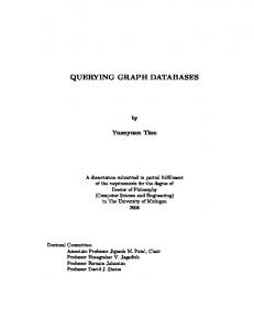
In order to be scalable, we developed our framework using the actor model. The actor model is an alternative to thread or process-based programming for building concurrent applications. In this model, an application is organized as a set of computational units called actors, that run concurrently and communicate together in order to solve a given problem. We built GDB using AKKA14 , a Scala framework that allows building distributed applications using the actor model. As shown in Figure 2, GDB uses four types of actors, each running on different machines: the server, that creates, loads and shuts down the graph databases, the master client, that executes traversal workloads and manages a series of slave clients, whose role is to send many basic requests to the graph database in parallel, and the benchmark runner, that executes benchmarks and thus attributes workloads to the master client and the server. The main responsibility of the server is to host the graph databases. More precisely, the server executes load workloads assigned by the benchmark runner. It has thus the responsibility to measure the time needed to load the databases with randomly generated datasets. When each database is loaded, it starts a Rexster server in order to make the database accessible remotely to the clients. The first role of the master client is to execute and measure the time required to perform traversal workloads. Moreover, the master client also measures the time required to perform intensive workloads. These intensive workloads are not directly executed by the master client but split into parts. Then, all these workload parts will be assigned to different client threads and all executed in parallel. In order to do that, the master client has at its disposal a client-thread pool that will be used to execute parts of intensive workloads. However, the responsibility of the master client for intensive workloads is limited to measuring the time required to get an answer from all the clients assigned to the intensive workload and does not take part to the workload execution. This client-thread pool is provided by a series of slave clients: each of these slaves obeys the master client and controls a series of client-threads. The number of threads controlled by a slave is equal to the number of cores available on the machine on which they are executed. For example, if the slave client runs on a two-cores machine, the slave client will control at most two concurrent threads, so that we are sure that the threads are really executed in parallel by the slave. Moreover, the slave clients are also centrally controlled and synchronized by the master client, so that each slave client starts its client-threads at approximately the same moment when performing an intensive workload. Finally, the benchmark runner plays the role of actors coordinator: it receives as input a benchmark defined by the user and assigns workloads to the server or the master client accordingly. Finally, it also logs and stores the measures returned. The communication between the clients and the databases is made using two different communication mechanisms depending on the type of workload executed: 14 http://www.akka.io
•
We used the embedded version of each database. Particularly, Titan-Cassandra also uses Cassandra in embedded mode, which allows to increase the performance, as Titan and Cassandra are running on the same JVM. Moreover, for this configuration, Cassandra is configured to run on one single node.
•
In order not to favor one database over another, we have not done any performance tuning specifically for a database: we left the settings with the default value.
B. Load workload 1) Benchmarking conditions: The workloads were executed using the following settings:
Fig. 2.
•
•
All the datasets were randomly generated using a scale-free network generator based on the BarabasiAlbert model [1] using a mean node degree set to five. The graphs generated using this model are characterized by a power-law degree distribution with a preferential attachment: the more a node is already connected, the more likely it will be connected to new neighbors. Each graph vertex got a string property.
•
Each database was configured in batch loading mode for loading the datasets. In this mode, the database uses one single thread to load the dataset.
•
Each vertex inserted is also indexed on its unique property.
GDB Actor System
For intensive workloads, the clients communicate with the Rexster server using Rexster’s REST API, as it simply leaded to better and more stable performances. As REST requests are self-contained, they are executed as a single transaction by the databases. Rexpro is used during traversal workload, as, contrary to REST communication, this protocol offers the possibility to make a Gremlin traversal script directly executed by the database and not by the client. This scheme leads to better performances, as it reduces drastically the number of messages exchanged between the client and the Rexster server during the traversal. IV.
R ESULTS
In this section, we present the measures obtained when using GDB on four graph databases: Neo4j, DEX, Titan and OrientDB. In order to analyze the impact of the graph size on the performances of the databases, traversal and intensive workloads were executed on two graph sizes: first 250,000 (approx. 1,250,000 edges) and 500,000 vertices (approx 2,500,000 edges). Although we only included the figures that concern the bigger graph, we will mention the measures obtained on the smaller graph when they significantly differ. A. Experimental setup •
We ran the Server actor (and therefore the graph databases) on a 2.5Ghz dual core machine with 8G of physical memory (5G allocated to the process) and a standard hard disk drive (non-SSD).
•
All the clients actors (both the Master Client and the Slave Clients) were executed on a 2.5Ghz single core with 2G of physical memory computers.
•
•
All the machines are located on the same local area network.
2) Results: Figure 3 shows the evolution of the insertion time during the loading process of a randomly generated social network dataset composed of approximatively 3,000,000 graph elements (500,000 vertices and approx. 2,500,000 edges). We opted for this size for two reasons. First, we think that 500,000 vertices is enough to model already interesting problems (for example, June 1, 2013, the graph of co-purchasing Amazon items was composed of 403.394 vertices and 3,387,388 edges15 ). Secondly, after that point, the loading time became quite significant, specifically for one of the databases tested. We used two different buffer sizes for loading the databases. Like mentioned earlier, this buffer size simply indicates the number of vertices/edges inserted before committing a transaction, and thus, the number of elements inserted in the database before flushing to the disk. As shown in Tables I and II, using a bigger buffer leads to better performances for almost all databases. Using a buffer size of 20.000 elements, Neo4j in particular took two times less time to fully load the dataset than using a buffer size of 5.000. Indeed, using a larger buffer allows the database to access the hard disk drive less often during the loading process. Therefore, the time needed to load the dataset is reduced. The conclusion is the same for DEX, Titan-BerkeleyDB and TitanCassandra, but the impact of the increased buffer size is less important. The measures obtained with OrientDB does not seem to be impacted by the buffer size: the loading rate for this database is always much lower than the other candidates. From Figure 3, we can see that, regardless the buffer size used, the loading time is increasing approximatively linearly 15 http://snap.stanford.edu/data/amazon0601.html
TABLE I. 500
Neo4j DEX Titan-BDB Titan-Cassandra OrientDB
400 Time (seconds)
L OAD WORKLOAD RESULTS ( SEC .) USING A BUFFER SIZE OF 5,000
Load Workload with a 5,000 buffer size Graph el. loaded 500k 1000k 1500k 2000k 2500k 3000k
300
200
TABLE II.
Neo4j
DEX
Titan-BDB
Titan-Cassandra
OrientDB
5.74995 12.04847 16.98259 22.15680 33.10645 297.87892
19.44911 32.03252 51.85323 66.73069 82.25261 99.1784
18.53484 33.23480 50.31449 65.55982 80.15614 94.44010
52.51524 81.62522 115.72004 139.48701 178.41247 215.78923
56.75998 588.83879 1005.19257 1359.54699 1986.79631 4350.20323
L OAD WORKLOAD RESULTS ( SEC .) USING A BUFFER SIZE OF 20,000
100
0
0
500000
1e+06 1.5e+06 2e+06 Graph elements inserted
2.5e+06
3e+06
(a)
DEX
Titan-BDB
Titan-Cassandra
OrientDB
3.98751 8.25654 11.06476 14.02776 18.81234 143.57329
19.06939 30.99353 44.76818 64.67971 79.394 95.60929
19.52635 31.43026 44.60898 55.74031 66.35664 77.19206
50.56084 80.49548 118.12311 144.46303 171.19640 206.45922
54.59390 588.90165 1010.05765 1388.35480 1808.26900 5552.70849
C. Traversal workloads
Neo4j DEX Titan-BDB Titan-Cassandra OrientDB
400
1) Benchmarking conditions: The workloads were executed using the following settings:
300
•
All the databases are loaded with the same graph before starting to execute the workloads.
200
•
We did 100 measures for each traversal workload, selecting each time a different source vertex (and destination vertex for the shortest path workload).
•
We have limited the number of results (ie. number of paths returned for the shortest path workload and the number of vertices returned for the neighborhood exploration workload) evaluated when executing the traversal workloads to 3,000. It was particularly required for the shortest path workload, as the number of paths between two randomly selected vertices may potentially be really high if the source and/or the destination vertex is strongly connected.
100
0
0
500000
1e+06 1.5e+06 2e+06 Graph elements inserted
2.5e+06
3e+06
(b) Fig. 3. buffer
Neo4j
Load Workload with a 20,000 buffer size
500
Time (seconds)
Graph el. loaded 500k 1000k 1500k 2000k 2500k 3000k
Load workload using a (a) 5,000 and (b) 20,000 graph elements
for DEX, Titan-BerkeleyDB and Titan-Cassandra. Concerning Neo4j, graph elements were inserted at a constant rate until a specific moment when the insertion speed tumbled. This phenomenon can clearly be observed in Figure 3(a): the time measured after inserting the 2,500,000th graph element was 33.1 seconds, while inserting 10,000 additional elements took up to 83.4 seconds, making the 2,510,000th graph element inserted after 116.5 seconds. After that point, the loading time continued to increase linearly until the phenomenon reappeared later. This does not seem to be linked to the buffer size, as the phenomenon seems to happen randomly. Our hypothesis is that this is due to a background daemon (probably related to data reorganization on disk) that starts at a specific moment when loading the dataset. Concerning OrientDB, the loading time is growing linearly at the beginning, but starts to increase more rapidly at always approximatively the same moment (after having inserted between the 520,000th and 550,000th graph element). This phenomenon reappeared later during the loading process between the 2,300,000th and 2,600,000th graph element inserted (not visible in the figure).
2) Shortest path workload: Figure 4 summarizes the results obtained by each database with four different configurations of the shortest path workload (using 2, 3, 4 and 5 hops limits). We can see that Neo4j outmatches all the other candidates, with a mean and median time always inferior to the other databases. It is also the database that had the most predictable behavior with a much lower results variance than the other candidates. Based on the same figure, it is clear that Titan-Cassandra is much slower than the other solutions for this workload, as its mean and median measures are always superior to the other databases. Moreover, its results are generally much more fluctuating than the other candidates: as shown in Figure 4, orange boxes are always taller than the other boxes. Its results variance follows the same trend. Concerning DEX and OrientDB, they obtained at first sight equivalent results: sometimes the former obtained better performances, while the latter outperformed DEX in other situations. However, by looking at the results more closely, we noticed that OrientDB obtained in general better performances than DEX but sometimes got really poor results that strongly influenced the mean value. Indeed, the results variance
Fig. 4. Shortest path workload on a 500,000 vertices graph Boxes contain all the values between first (Q1) and third quartile (Q2). Bold points represent the mean measure, horizontal bar inside boxes the median measure and horizontal bar outside boxes regular (non-outlier) maximum or minimum values. Outliers are computed using the formula M axOutlierT hreshold = Q3 + (InterQuartileRange ∗ 1.5) and M inOutlierT hreshold = Q1 − (InterQuartileRange ∗ 1.5) and represented as small circles (two small circles if outliers overlap). Maximum farouts values are computed using the formula M axF aroutT hreshold = Q3 + (InterQuartileRange ∗ 2) and represented as triangles.
observed for OrientDB is generally much higher than what we observed for the other databases. Finally, we conclude that the hops limit does not really seem to influence the results: the above conclusions are valid regardless the number of hops used. 3) Breadth first exploration of nodes neighborhood workload: The results obtained for this workload confirm our previous analysis: as shown in Figure 5, Neo4j gets the best results, while Titan-Cassandra is still way behind the other solutions. We also see that the performances of OrientDB are again particularly unstable. Indeed, the database obtained good results with a 1 and 2 hops limit but they totally crumbled for the last workload configuration. Particularly, the maximal time recorded for OrientDB during this workload is up to 15 times higher than the maximal result obtained by Neo4j. Moreover, the memory consumption of OrientDB seems to be more significant that the other databases, as it is the only candidate that ran out of memory when we tried a four hops limit. D. Intensive workloads 1) Get vertices by ID intensive workload: Similarly as for traversal workloads, we did 100 measures for each intensive workload execution. At first sight, we notice in Figure 6 that the shape of the curves are all very similar: the performance increase is relatively important (between +100 % and +120%) when we switch from one to two concurrent clients to perform the workload. Then, this increase becomes less and less important to be finally almost inexistent for the transition from three to four concurrent clients.
Fig. 5.
Neighborhood exploration workload on a 500,000 vertices graph
The reason is simple: as the databases are running on a dual core machine, they can serve up to two clients “really” in parallel. Therefore, the time required to execute the same number of request is almost halved when performed by two concurrent clients. Then, if an additional client joins and starts to send requests to the database, the latency is likely to increase for the two previous clients. This is exactly what happens here, except that the time required to complete the workload does not immediately start to increase when we execute it with more than two concurrent clients. Again, the explanation is simple. Indeed, although the clients are executed really in parallel, they do not keep constantly the database busy, as for each request, the client has to wait a result before sending a new request. During the time interval between the moment when it sends an answer to a client and when it receives a new request from this client, the database can possibly handle a request from an additional third client. Again, we observe that Titan-Cassandra offers lower performances than the other databases, regardless the number of clients used to perform the workload. The results obtained by the other databases are really close. Moreover, we observe in Figure 6 that the gap between the databases narrows as the number of clients increases. By only looking at the previous figure, it is quite hard to determine which database got the best results for this workload, particularly with four clients. However, by looking at Table III, we observe that DEX and OrientDB outperform Neo4j and TitanBerkeleyDB. Determining which database between between DEX and OrientDB is the most adapted for this workload is not an easy task, as they obtained really close results. The only criteria that can be used to differentiate the two implementations is the results dispersion. Indeed, similarly as the previous workloads, we observe in Table III that the results variance and maximal measure of OrientDB are respectively 4748 and 385 % higher than the same measures obtained by DEX.
Neo4j DEX Titan-BDB Titan-Cassandra OrientDB
0.4 0.35 Time (seconds)
TABLE IV. G ET VERTICES BY PROPERTY INTENSIVE WORKLOAD RESULTS ( SEC .) WITH 4 CLIENTS DOING 200 OPS TOGETHER ON A 500.000 VERTICES GRAPH
Get vertices by ID intensive workload
0.45
Neo4j DEX Titan-BDB Titan-Cassandra OrientDB Mean 0.222720 0.233231 0.235028 0.302582 0.218648 Median 0.219277 0.226657 0.230678 0.299175 0.217392 Variance 0.000424 0.000601 0.001383 0.000287 0.000094 Min. 0.203823 0.210744 0.207254 0.282349 0.200086 Max. 0.385821 0.419826 0.590591 0.383336 0.249710
0.3 0.25 0.2 0.15 0.1 1
1.5
2
2.5 Number of clients
3
3.5
4
Fig. 6. Get vertices by ID intensive workload on a 500,000 vertices graph Each point represents the average time to get an answer for 200 GET vertex by ID requests performed by X clients (each client sends 200/X requests).
Neo4j DEX Titan-BDB Titan-Cassandra OrientDB
20 Time (seconds)
0.05
Add edges intensive workload
25
TABLE III. G ET VERTICES BY ID INTENSIVE WORKLOAD RESULTS ( SEC .) WITH 4 CLIENTS DOING 200 OPS TOGETHER ON A 500.000
15
10
5
VERTICES GRAPH 0
Neo4j DEX Titan-BDB Titan-Cassandra OrientDB Mean 0.094484 0.092099 0.095918 0.129590 0.097085 Median 0.089267 0.090383 0.090163 0.123343 0.084364 Variance 0.000480 0.000128 0.000514 0.000255 0.006205 Min. 0.076205 0.079224 0.081593 0.113491 0.074536 Max. 0.242574 0.177440 0.272045 0.204182 0.859757
2) Get vertices by property intensive workload: The purpose of this workload is to evaluate the indexing mechanism provided by each database. The first thing we observe in Figure 7 is that all the curves have the same shape. However, they all are flatter than previously. Indeed, while the performance increase between using one and two clients during the previous workload was between +100 % and +120%, here the increase is between +85 % and +90 %. Here again, we observe that Titan-Cassandra is way behind the other solutions. Then, similarly as the previous workload, the other databases results are pretty close but this time the two databases that stand out are Neo4j and OrientDB. Here, as shown in Table IV, the latter did not suffer from variable results so we can not differentiate the two databases on this criteria.
Get vertices by property intensive workload
1
Neo4j DEX Titan-BDB Titan-Cassandra OrientDB
0.9
Time (seconds)
0.8 0.7 0.6 0.5 0.4 0.3 0.2
Fig. 7. graph
1
1.5
2
2.5 Number of clients
3
3.5
4
Read vertices by property intensive workload on a 500,000 vertices
Fig. 8.
1
1.5
2
2.5 Number of clients
3
3.5
4
Add edges intensive workload on a 500,000 vertices graph
3) Add edges intensive workload: This workload is totally different as it no more only requires to read the database but also to write (insert) data. Transactions were activated for all the databases during the workload. Note that communicating with the Rexster server using REST does not allow to control how and when transactions are committed: the server itself automatically commits transactions. First, we observe in Figure 8 that the curves are all quite different: they are decreasing for DEX, Titan-Cassandra and Titan-BerkeleyDB and increasing for OrientDB, meaning that the first three scale much better when the number of clients writing simultaneously the database increases. Concerning Neo4j, we can see that its results do not seem to be influenced by the number of clients. We also observe that the results obtained by Neo4j, TitanBerkeley DB and OrientDB are much inferior to those obtained with DEX and Titan-Cassandra. This is likely linked to the transaction mechanism that limits the number of clients concurrently adding records in the database. We tried to tune the settings to improve that situation but did not succeed: Neo4j and OrientDB really seem to complain for this type of operation. Moreover, the results obtained by OrientDB varied much more than the other databases. Particularly, the gap between the minimal and maximal measure observed is quite huge. Finally, which database between DEX and Titan-Cassandra got the best performances? We observe in Figure 8 that the behavior of the two databases is similar: they scale really well when the number of clients increases. However, by looking at Table V more closely, we observe that DEX always obtained the best results. 4) Write properties intensive workload: This workload differs from the previous one as it implies to modify vertices
TABLE V.
A DD EDGES INTENSIVE WORKLOADS RESULTS ( SEC .) ON A 500,000 VERTICES GRAPH
1 client 2 clients 3 clients 4 clients DEX Titan-C DEX Titan-C DEX Titan-C DEX Titan-C Mean 0.783084 1.100030 0.430438 0.610036 0.308893 0.455871 0.271001 0.392483 Median 0.782582 1.091260 0.426864 0.605103 0.307174 0.445380 0.271813 0.392073 Variance 0.000658 0.008100 0.000558 0.000314 0.000084 0.003657 0.000176 0.000500 Min. 0.721273 0.938597 0.406419 0.577281 0.290249 0.410409 0.247047 0.354945 Max. 0.972766 1.751364 0.648427 0.646169 0.337645 0.955497 0.309281 0.440967
GET vertices by ID and UPDATE intensive workload
70
As GDB was developed as a framework, we plan to improve and extend the tool in the future. For example, it might be really interesting to add new traversal workloads such as centrality or graph diameter computation workloads to the tool.
Neo4j DEX Titan-BDB Titan-Cassandra OrientDB
60 50 Time (seconds)
best results with traversal workloads is definitely Neo4j: it outperforms all the other candidates, regardless the workload or the parameters used. Concerning read-only intensive workloads, Neo4j, DEX, Titan-BerkeleyDB and Orient achieved similar performances. However, for read-write workloads, Neo4j, Titan-BerkeleyDB and OrientDB’s performances degrade sharply. This time DEX and Titan-Cassandra take their game with much more interesting results than the other databases.
40
VI.
30
This work was done in the context of a master’s thesis supervised by Peter Van Roy in the ICTEAM Institute at UCL.
20 10 0
ACKNOWLEDGMENTS
1
1.5
2
2.5 Number of clients
3
3.5
R EFERENCES
4
Fig. 9. Write properties intensive workload results (sec.) on a 500,000 vertices graph
properties and thus also to update the index. However, many conclusions from the previous workload still apply here. As shown in Figure 9, the behavior of Neo4j does not seem to be dependent on the number of concurrent clients, while the measurements for OrientDB are again really variant. However, its performances are globally superior compared to the previous workload. Concerning the three other databases, Titan-BerkeleyDB gets this time better results, while Titan-Cassandra and DEX still obtain the best performances. Again, these two databases scale really well when the number of clients increases. As shown in table VI, DEX still obtained the best performances compared to the other solutions, with a lower mean and median measures and more stable results.
[1] [2] [3] [4] [5]
[6] [7] [8] [9]
V.
C ONCLUSION
We presented GDB, an extensible tool to compare different Blueprints-compliant graph databases. We used GDB to compare four graph databases: Neo4j, DEX, Titan (BerkeleyDB and Cassandra) and OrientDB (local) on different types of workloads, each time identifying which database was the best and the less adapted. Based on our measure, the database that obtained the TABLE VI.
W RITE PROPERTIES INTENSIVE WORKLOADS RESULTS ( SEC .) ON A 500,000 VERTICES GRAPH
1 client 2 clients 3 clients 4 clients DEX Titan-C DEX Titan-C DEX Titan-C DEX Titan-C Mean 0.552040 0.855709 0.299732 0.449373 0.216897 0.337556 0.189509 0.306128 Median 0.548127 0.835181 0.295415 0.438381 0.216063 0.314306 0.187603 0.292751 Variance 0.000686 0.011076 0.000855 0.000469 0.000049 0.011797 0.000134 0.003635 Min. 0.508350 0.736268 0.279791 0.420570 0.202632 0.301302 0.170240 0.266679 Max. 0.617997 1.542111 0.579817 0.501984 0.232145 1.396984 0.226531 0.824158
Reka Albert Albert-Laszlo Barabasi. Emergence of scaling in random networks. Science, 286:509–512, 1999. Renzo Angles. A comparison of current graph database models. Third International Workshop on Graph Data Management: Techniques and Applications, 2012. Claude Berge. Graphs and Hypergraphs. Elsevier Science Ltd, 1985. M. L. Brodie O. Erling C. Bizer, P. A. Boncz. The meaningful use of big data: four perspectives - four challenges. SIGMOD Record, 40. D. Dominguez-Sal, P. Urbon-Bayes, A. Gimenez-Vano, S. GomezVillamor, N. Martinez-Bazan, and J.L. Larriba-Pey. Survey of graph database performance on the hpc scalable graph analysis benchmark. In Proceedings of the 2010 international conference on Web-age information management, July 2010. T. Walsh L. Antsfeld. Finding multi-criteria optimal paths in multi-modal public transportation networks using the transit algorithm. In Intelligent Transport Systems World Congress, October 2012. B. Andreopoulos M. Schroeder L. Royer, M. Reimann. Unraveling protein networks with power graph analysis. PLoS Computational Biology, July 2008. Ladialav Hluchy Marek Ciglan, Alex Averbuch. Benchmarking traversal operations over graph databases. 2012 IEEE 28th International Conference on Data Engineering Workshops, 2012. D. Ritter. From network mining to large scale business networks. WWW (Companion Volume), pages 989–996, 2012.