Thresholding Methods for Fisher's Classifier ... Fisher's classifier, obtains the threshold by computing ... minimizing the classification error in the transformed.
An Empirical Evaluation of the Classification Error of Two Thresholding Methods for Fisher’s Classifier Luis Rueda and Alioune Ngom School of Computer Science University of Windsor Windsor, ON, N9B 3P4, Canada. E-mail: {lrueda,angom}@uwindsor.ca Abstract In this paper, we empirically analyze two methods for computing the threshold in Fisher’s classifiers. One of these methods, which we call FC∧ or traditional Fisher’s classifier, obtains the threshold by computing the middle point between the two means in the projected space. The second method, which we call FC+ , obtains the threshold by computing the optimal classifier in the transformed space. We conduct the analysis in widely used public datasets for cancer detection and protein classification. The empirical results show that FC+ leads to smaller classification error than FC∧ . The results on Cancer data demonstrate that minimizing the classification error in the transformed space leads to smaller classification error in the original multi-dimensional space. As opposed to this, the results on protein classification show that selecting the theshold that minimizes the error in the transformed space, assuming the data is normally distributed, does not necessarily lead to the best classifier.
1
Introduction
The study of linear classifiers has been a very important problem in the field of statistical pattern recognition in the past few decades. In many applications, linear classifiers are preferred because of their classification speed and their simplicity in the implementation. We consider two data sets containing labeled samples, D1 = {x11 , x12 , . . . , x1n1 } and D2 = {x21 , x22 , . . . , x2n2 }, where x1j and x2j are drawn independently from their respective classes, namely ω1 and ω2 respectively. The aim is to find a linear function, g(x) = wt x + w0 = 0 , (1) that classifies an object, represented by a realvalued vector, x = [x1 , . . . , xd ]t , into the respective
class, where w is a d-dimensional weight vector, and w0 is a threshold weight. We consider two classes, ω1 and ω2 , which are represented by two normally distributed d-dimensional random vectors, x1 ∼ N (µ1 , Σ1 ) and x2 ∼ N (µ2 , Σ2 ). Thus, the statistical information about the classes is determined by the mean vectors, µ1 and µ2 , and the covariance matrices, Σ1 and Σ2 . Various schemes that yield linear classifiers have been reported in the literature, including Fisher’s classifier [5, 18, 19], the perceptron algorithm (the basis of the back propagation neural network learning algorithms) [6, 8, 11, 12], piecewise recognition models [9], random search optimization [10], removal classification structures [1], adaptive linear dimensionality reduction [7] (which outperforms Fisher’s classifier for some data sets), linear constrained distance-based classifier analysis [4] (an improvement to Fisher’s approach designed for hyperspectral image classification), and recursive Fisher’s discriminant [3]. Rueda and Oommen [15, 16] have recently shown that the optimal classifier between two normally distributed classes can be linear even when the covariance matrices are not equal. They showed that although the optimal classifier for normally distributed random vectors is a second-degree polynomial, it degenerates to be either a single hyperplane or a pair of hyperplanes. In [14], a new approach to selecting the best hyperplane classifier (BHC), which is obtained from the optimal pairwise linear classifier, was introduced. It is shown that, on synthetic data, the BHC is twice as fast as the pairwise linear classifier, and attains nearly optimal classification, outperforming Fisher’s classifier on two-dimensional normally distributed random vectors. However, the BHC only applies to two-dimensional feature spaces, and its implementation to spaces of more than three dimensions is far from trivial, for two reasons: the conditions for the BHC are highly restric-
tive, and solving the constrained optimization problem requires a time-consuming numerical solution. In this paper, we empirically analyze two different approaches used to optimize the threshold selection procedure in linear classifiers when multi-dimensional samples are projected onto the one-dimensional space. One of these methods, which we call FC∧ or traditional Fisher’s classifier, obtains the threshold by computing the middle point between the two means in the projected space. The second method, which we call FC+ , obtains the threshold by computing the optimal classifier in the transformed space [13]. We conduct the analysis in the Wisconsin Diagnostic Breast Cancer dataset, and in the classification of ’kinase’ and ’ras’ superfamily of proteins from the Protein Information Resource database.
2
Fisher’s Classifier
The basic idea of Fisher’s classifier is to find an efficient linear transformation that provides the best separability between the classes. We consider the case in which the samples are transformed onto the onedimensional space and the number of classes is two. A more detailed discussion about the general scenario for more than two classes can be found in [5, 18, 19]. Thus, in our case, the linear transformation is seen as a projection of the points from the d-dimensional space onto the line determined by (1). Suppose that we are given D1 = {x11 , x12 , . . . , x1n1 } and D2 = {x21 , x22 , . . . , x2n2 } drawn from the corresponding classes, ω1 and ω2 , whose a priori probabilities are P (ω1 ) and P (ω2 ) respectively. Projecting D1 and D2 onto a line produces D1′ = {y11 , y12 , . . . , y1n1 } and D2′ = {y21 , y22 , . . . , y2n2 }, where yik = wt xik with i = 1, 2 and k = 1, . . . , ni . The aim is to find a vector, w, which leads to the maximum class separability in the projected space. To derive Fisher’s classifier, we first define the sample mean of the projected data as follows:
µ ˜i =
ni ni 1 X 1 X yik = wt xik = wt µi , ni ni k=1
(2)
σ ˜i2
=
ni X
(yik − µ ˜i ) =
k=1
ni X
wt xik − wt µi
k=1
�2
= wt Si w , (3)
where Si =
ni X
(xik − µi )(xik − µi )t
(4)
k=1
is the scatter matrix for ωi . The aim of Fisher’s approach is to maximize the separability between the classes in the projected line, which is given by the following criterion function: 2
J(w) =
(˜ µ1 − µ ˜2 ) , σ ˜12 + σ ˜22
(5)
Using the definitions of (2) and (3), J(·) can be written as follows: J(w) =
wt SB w . wt SW w
(6)
where SW = S1 +S2 is the within-class scatter matrix, and SB = (µ1 − µ2 )(µ1 − µ2 )t is the between-class scatter matrix. The solution for the vector w that maximizes (6) is given by: w = S−1 W (µ1 − µ2 ) .
(7)
To complete the linear classifier, the threshold w0 has to be obtained. The two approaches that are compared in this paper are briefly discussed in the next section.
3
Computing the Threshold
A simple approach to compute the threshold, which we call FC∧ , is to assume that the distributions in the original space have identical covariance matrices, and take the independent term of the optimal quadratic classifier, which results in:
w0∧ =
k=1
where µi is the sample mean of the original data, obtained by applying the maximum likelihood estimation (MLE) method. Similarly, the sample scatter for the projected data is defined as follows:
2
= = =
P (ω2 ) 1 (8) − (µ1 + µ2 )t S−1 W (µ1 − µ2 ) − log 2 P (ω1 ) P (ω2 ) 1 (9) − (µ1 + µ2 )t w − log 2 P (ω1 ) P (ω2 ) 1 (10) − (wt µ1 + wt µ2 ) − log 2 P (ω1 ) 1 P (ω2 ) − (˜ µ1 + µ ˜2 ) − log . (11) 2 P (ω1 )
This implies that the threshold is obtained as the middle point between the two means in the projected line, shifted by the logarithm of the ratio between the a priori probabilities of the classes. It is important to observe that choosing the threshold as the middle point between the two means in the transformed space may lead to an inefficient classification scheme for some situations. In [13], a more efficient approach has been introduced, which selects the threshold as the value in which the one-dimensional distribution functions in the projected line are equal, i.e. by applying the optimal Bayesian classifier in the transformed space. As observed in [13], there are situations in which Fisher’s classifier with the threshold obtained as in (8) produces a classifier that is quite distant from the optimal quadratic classifier in the area of the hyperquadric in which the samples are more likely to occur. This leads to a poorer linear classifier, which can be enhanced by adjusting the threshold in the projected line. Thus, a more efficient approach to obtain that threshold, namely FC+ , which is derived from the optimal Bayesian classifier in the transformed space. Let x1 ∼ N (µ1 , Σ1 ) and x2 ∼ N (µ2 , Σ2 ) be two normally distributed random vectors that represent the two classes ω1 and ω2 , whose a priori probabilities are P (ω1 ) and P (ω2 ) respectively. From (2), we know that the means in the projected line are obtained as follows: µ ˜ i = w t µi ,
(12)
and from (3), the variances are obtained as follows: σ ˜i2 = wt Σi w .
(13)
FC+ computes the threshold for Fisher’s classifier, and, in general, for any linear classifier1, as the optimal decision boundary in the projected line. Let x1 ∼ N (˜ µ1 , σ ˜12 ) and x2 ∼ N (˜ µ2 , σ ˜22 ) two normally distributed random variables, where µ ˜i and σ ˜i2 are the mean and variance of xi , which are obtained as in (12) and (13) respectively. In this scenario, the optimal Bayesian classifier is computed as the point(s) in which the conditional a posteriori probabilities of the two classes are equal. Thus, substituting these probabilities by the corresponding normal distribution density function, taking natural logarithm on both sides, 1 Although FC+ is based on Fisher’s classifier, it can be generalized to any linear classifier which projects multi-dimensional random vectors onto the one-dimensional space. The generalization is achieved by selecting different instantiations for the vector w in (12) and (13).
and other algebraic manipulations, we obtain the optimal quadratic classifier as follows: � � � � 1 1 1 µ ˜2 µ ˜1 2 − 2 x + − 2 x+ 2 σ ˜2 σ ˜1 σ ˜12 σ ˜2 � 22 � 2 2 1 µ ˜2 µ ˜ σ ˜ P (ω1 ) − 21 + log 22 + log 2 σ ˜22 σ ˜1 σ ˜1 P (ω2 )
= 0 (14)
This polynomial has two roots, which may be identical, leading to a single solution. Two mutually exclusive and exhaustive cases for σ ˜1 and σ ˜2 are possible. • σ ˜1 = σ ˜2 = σ ˜ : In this case, the second-degree polynomial of (14) becomes the following linear function on x: � � µ ˜22 − µ ˜21 P (ω1 ) µ ˜1 − µ ˜2 x + + log = 0, (15) 2 2 σ ˜ 2˜ σ P (ω2 ) where the solution for x is given by: (ω1 ) µ ˜21 − µ ˜ 22 − 2˜ σ 2 log P P (ω2 )
2 (˜ µ1 − µ ˜2 )
(16)
.
• σ ˜1 6= σ ˜2 : In this case, the second-order degree polynomial on x has two solutions, given by: � � r� � � � µ ˜2 σ ˜22
−
µ ˜1 σ ˜12
±
µ ˜ 1 −˜ µ2 σ ˜1 σ ˜2
1 σ ˜22
2
+2
−
1 σ ˜22
−
1 σ ˜12
P (ω1 ) log σσ˜˜21 P (ω2 )
1 σ ˜12
(17) Given the values of the two roots of the secondorder degree polynomial, select the threshold to be the root that falls between the two means in the transformed space, as follows: w0+
4
= =
−x+ if µ ˜1 < x+ < µ ˜2 or µ ˜2 < x+ < µ ˜1 −x− otherwise
Experiments on the Cancer Data
In order to test the accuracy of the two threshold selection approaches, we performed some simulations using the Wisconsin Diagnostic Breast Cancer (WDBC) dataset obtained from the UCI machine learning repository2 . This dataset contains samples drawn from two classes, the “benign” and the “malignant” classes. To evaluate the classifiers, we have followed the ten-fold cross validation approach, utilizing, first, the majority of the samples (315 and 189 for the benign and malignant classes respectively) to train 2 http://www.ics.uci.edu/˜mlearn/MLRepository.html.
of samples ‘M’ Total 189 504 162 432 144 387 126 333 108 252 90 216 72 171 63 153 72 144 54 126 45 99
Classification error FCˆ FC+ Diff. 4.8095 3.0952 1.7143 5.0556 4.2778 0.7778 5.6829 4.7917 0.8912 6.3665 5.4503 0.9161 8.0208 6.6667 1.3542 8.1429 6.5000 1.6429 9.3182 7.1023 2.2159 8.3571 6.9286 1.4286 6.2500 5.0000 1.2500 7.9167 7.7083 0.2083 27.2917 26.2500 1.0417
Table 1: Empirical results obtained after performing simulations on real-life data obtained from the WDBC dataset. The classification errors represent the percentage of misclassified samples obtained from the average (for both classes) as per the ten-fold cross validation approach. the classifier. We then continued decreasing the number of training samples so that the effect of considering low cardinality datasets against the dimensionality of the feature space is observed. The classification error obtained from training and testing FCˆ and FC+ are shown in Table 1. The first and second columns list the number of training samples from the benign and malignant classes respectively, and the third column contains the total number of training samples used for both classes. The fourth and fifth columns contain the average classification error obtained after evaluating the classifier (as per the ten-fold cross validation approach). The last column contains the difference between the classification errors for FCˆ and FC+ . The results from the table show that FC+ leads to smaller classification errors than the FCˆ for all the training dataset sizes used. We also observe that the classification error is substantially small for all the cases, except for the last one, where we used 45 samples from the malignant class to train the classifier. This behavior is quite reasonable, since the dimensionality of the feature space is 30, which is slightly less than the number of training samples. To visualize the effect of reducing the training dataset cardinalities, the relationship between the size of the training datasets and the resulting classification error are plotted in Figure 1. The curve representing the classification error grows slowly up to size 72, and then decreases slowly up to size 54, to finally “slant-
30.00 FC^ FC+
25.00
Classification error
No. ‘B’ 315 270 243 207 144 126 99 90 72 72 54
20.00
15.00
10.00
5.00
0.00 189
162
144
126
108
90
72
63
72
54
45
Size of training dataset (Malignant)
Figure 1: Size of the training dataset for the malignant class versus classification error. The y-axis represents the classification error obtained after averaging the ten rounds from the ten-fold cross validation, while the xaxis shows the size of the training dataset representing the malignant class.
up” to a higher classification error for size 45. As can be observed in the figure, FC+ leads to smaller classification error than the FCˆ in all the cases. This behavior, again, corroborates the superiority of FC+ in real-life data.
5
Results on Protein Classification
In this section we analyze the performances of both threshold selection methods on the protein classification problem. The protein classification problem is defined as follows. Given a protein superfamily, F, and the sequence of an unknown protein, S, we want to determine whether S belongs to F or not. The solution to this problem is important in many aspects of bioinformatics and computational molecular biology. If the superfamily F of an unlabeled sequence S is determined, then one can infer the molecular structure and function of S —this is due to the fact that proteins in a superfamily share similarity in structure and function. For our purpose, we applied the two threshold selection approaches discussed in Section 3, namely FC∧ and FC+ , for classifying protein sequences into either “kinase” superfamily or “ras” superfamily. These two datasets were obtained from the International Protein Sequence Database [2], release 62, in the Protein Information Resource (PIR) database maintained at the National Biomedical Research Foundation (NBRF-
∧
FC FC+
Kinase 96.67 91.25
Ras 96.41 97.60
Average 96.54 94.43
800
Kinase 600
Table 2: Classification accuracy for the two threshold selection approaches FC∧ and FC+ . The results correspond to the two protein families used in the testing, which are kinase and ras.
400
Ras 200
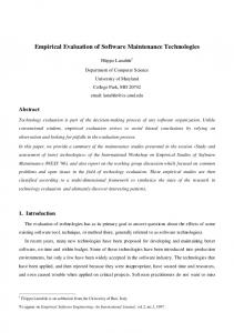
PIR) at the Georgetown University Medical Center3 . Since proteins are sequences of characters, we first applied the powerful protein feature extraction technique of [17] to obtain numeric data, which are then used in our classification approach. To evaluate the classifiers, we used 368 and 363 training samples respectively for kinase and ras (the test sets contain, respectively, 240 and 167). We have trained the two classifiers, FC∧ and FC+ , with the training sets, and tested them using the test sets. The results on classification accuracy (given in terms of percentage of correctly classified samples) are shown in Table 2. The rows in the table correspond to each of the aforementioned classifiers. The results show that both classifiers are very accurate for the “ras” superfamily, and that FC+ is less accurate for the “kinase” superfamily. If considering the average of classification accuracy for both classes, it is clear that FC∧ is more accurate (by more than 2%) than FC+ . This situation has not been observed in previous experiments, such as those of Section 4 and the ones on synthetic data discussed in [13], which show the opposite case. To analyze the results from a different perspective we have plotted the normal distribution probability density functions for the two classes, where the parameters of the distributions are obtained after transforming the training samples onto the one-dimensional space using the linear transformation y = wt x. The plot depicted in Figure 2 shows that the means in the projected space are very close to each other, and that the variance for “ras” is much larger than that of “kinase”. The thresholds for the two methods, FC∧ and FC+ , are also shown in the figure. Two observations are important here. First, from the theoretical point of view, since the variances are quite different from each other, it would be convenient to use two thresholds in FC+ : the points in which the two distribution functions intersect. Thus, the classification error would be minimized, assuming that the data projected onto the one-dimensional space obey the normal distribution. Second, from a practical perspective, it appears 3 Accessible
at http://pir.georgetown.edu.
0 −0.008
−0.006
−0.004
−0.002
0
0.002
w^
w+
0
0
0.004
0.006
Figure 2: Plot of the normal distribution probability density functions that correspond to the projected data (for classes kinase and ras) onto the onedimensional space (after the linear transformation). that the protein classification dataset obtained after the feature extraction method introduced in [17] does not obey the normal distribution, and hence the model for selecting a single approach based on the optimal Bayesian classifier in the transformed space does not provide the best option. The use of more than one threshold (not necessarily two) seems to be a better approach in this scenario. This is one of the open problems that deserve investigation.
6
Conclusions and Future Work
In this paper, we have presented an empirical comparison of two methods for obtaining the threshold in Fisher’s classifier. One of these methods, which we call FC∧ or traditional Fisher’s classifier, obtains the threshold by computing the middle point between the two means in the projected space. The second method, which we call FC+ , obtains the threshold by computing the optimal classifier in the transformed space. Our result on the WDBC dataset show that FC+ leads to smaller classification error than FC∧ for training datasets of different sizes. We also observe that the classification error increases substantially when the size of the training dataset decreases. The results on protein family classification show a scenario in which FC∧ is superior to FC+ . This thus corroborates that, in real-life data, the use of a single threshold (even it is the optimal in a theoretical sense) does not lead to the best classifier.
A problem that is related to our study, and that deserves investigation is the analysis of the classification error on d-dimensional normally distributed random vectors, where d > 4. The problem is far from trivial as it involves integrating the multivariate normal distribution density function. Another problem that deserves investigation is to consider situations involving more than two classes. In this case, the linear transformation suggested by Fisher’s approach (and, in general, by any linear classifier) involves a matrix instead of a vector, and leads to a d′ -dimensional space where d′ > 1. Acknowledgments: The authors’ research is partially supported by NSERC, the Natural Sciences and Engineering Research Council of Canada.
[8] O. Murphy. Nearest Neighbor Pattern Classification Perceptrons. In Neural Networks: Theoretical Foundations and Analysis, pages 263–266. IEEE Press, 1992. [9] A. Rao, D. Miller, K. Rose, , and A. Gersho. A Deterministic Annealing Approach for Parsimonious Design of Piecewise Regression Models. IEEE Transactions on Pattern Analysis and Machine Intelligence, 21(2):159–173, 1999. [10] S. Raudys. On Dimensionality, Sample Size, and Classification Error of Nonparametric Linear Classification. IEEE Transactions on Pattern Analysis and Machine Intelligence, 19(6):667–671, 1997.
References
[11] S. Raudys. Evolution and Generalization of a Single Neurone: I. Single-layer Perception as Seven Statistical Classifiers. Neural Networks, 11(2):283– 296, 1998.
[1] M. Aladjem. Linear Discriminant Analysis for Two Classes Via Removal of Classification Structure. IEEE Trans. on Pattern Analysis and Machine Intelligence, 19(2):187–192, 1997.
[12] S. Raudys. Evolution and Generalization of a Single Neurone: II. Complexity of Statistical Classifiers and Sample Size Considerations. Neural Networks, 11(2):297–313, 1998.
[2] W.C. Barker, J.S. Garavelli, H. Huang, P.B. McGarvey, B. Orcutt, G.Y. Srinivasarao, C. Xiao, L.S. Yeh, R.S. Ledley, J.F. Janda, F. Pfeiffer, H.W. Mewes, A. Tsugita, and C.H. Wu. The Protein Information Resource (PIR). Nucleic Acid Research, 28(1):41–44, 2000. [3] T. Cooke. Two Variations on Fisher’s Linear Discriminant for Pattern Recognition. IEEE Transations on Pattern Analysis and Machine Intelligence, 24(2):268–273, 2002. [4] Q. Du and C. Chang. A Linear Constrained Distance-based Discriminant Analysis for Hyperspectral Image Classification. Pattern Recognition, 34(2):361–373, 2001. [5] R. Duda, P. Hart, and D. Stork. Pattern Classification. John Wiley and Sons, Inc., New York, NY, 2nd edition, 2000. [6] R. Lippman. An Introduction to Computing with Neural Nets. In Neural Networks: Theoretical Foundations and Analsyis, pages 5–24. IEEE Press, 1992. [7] R. Lotlikar and R. Kothari. Adaptive Linear Dimensionality Reduction for Classification. Pattern Recognition, 33(2):185–194, 2000.
[13] L. Rueda. An Efficient Approach to Compute the Threshold for Multi-dimensional Linear Classifiers. Pattern Recognition, 37(4):811–826, April 2004. [14] L. Rueda. Selecting the Best Hyperplane in the Framework of Optimal Pairwise Linear Classifiers. Pattern Recognition Letters, 25(2):49–62, 2004. [15] L. Rueda and B. J. Oommen. On Optimal Pairwise Linear Classifiers for Normal Distributions: The Two-Dimensional Case. IEEE Transations on Pattern Analysis and Machine Intelligence, 24(2):274–280, February 2002. [16] L. Rueda and B. J. Oommen. On Optimal Pairwise Linear Classifiers for Normal Distributions: The d-Dimensional Case. Pattern Recognition, 36(1):13–23, January 2003. [17] J.T.L. Wang, Q. Ma, D. Shasha, and C.H. Wu. New Techniques for Extracting Features from Protein Sequences. IBM Systems Journals, 40(2):426– 441, 2001. [18] A. Webb. Statistical Pattern Recognition. John Wiley & Sons, N.York, second edition, 2002. [19] Y. Xu, Y. Yang, and Z. Jin. A Novel Method for Fisher Discriminant Analysis. Pattern Recognition, 37(2):381–384, February 2004.