kernel version of canonical correlation analysis (KCCA) ... of MAD in this study based on the established method known as kernel canonical correlation analysis.
ISPRS Annals of the Photogrammetry, Remote Sensing and Spatial Information Sciences, Volume III-1, 2016 XXIII ISPRS Congress, 12–19 July 2016, Prague, Czech Republic
KERNEL MAD ALGORITHM FOR RELATIVE RADIOMETRIC NORMALIZATION
Yang Bai a,b , Ping Tangb ,Changmiao Hu b,* a
b
University of Chinese Academy of Sciences, No.19A Yuquan Road, Beijing, China Institute of Remote Sensing and Digital Earth, Chinese Academy of Sciences, No.20 Datun Road, Beijing, China – (tangping, huchangmiao, baiyang) @radi.ac.cn Commission I, WG I/4
KEY WORDS : Relative radiometric normalization, multivariate alteration detection (MAD), canonical correlation analysis (CCA), kernel version of canonical correlation analysis (KCCA)
ABS TRACT: The multivariate alteration detection (M AD) algorithm is commonly used in relative radiometric normalization. This algorithm is based on linear canonical correlation analysis (CCA) which can analyze only linear relationships among bands. Therefore, we first introduce a new version of M AD in this study based on the established method known as kernel canonical correlation analysis (KCCA). The proposed method effectively extracts the non-linear and complex relationship s among variables. We then conduct relative radiometric n ormalization experiments on both the linear CCA and KCCA version of the M AD algorithm with the use of Landsat-8 data of Beijing, China, and Gaofen-1(GF-1) data derived from South China. Finally, we analyze the difference between the two methods. Results show that the KCCA-based M AD can be satisfactorily applied to relative radiometric normalization, this algorithm can well describe the nonlinear relationship between multi-temporal images. This work is the first attempt to apply a KCCA-based M AD algorithm to relative radiometric normalization.
1. INTRODUCTION As the growing need of multi-sensor, multi-temporal remote sensing data together used for land-use and land-cover change ( LUCC) monitoring, global resource environment analysis and climate change monitoring, relative radiometric normalization has practical significance for engineering applications. Relative radiometric normalization can establish the correction equation for each corresponding multi-spectral band in multi-temporal remote sensing data directly apply ing the pixel value of the image, without requiring any other parameters, such as atmospheric conditions on the day that remote sensing data obtained. Relative radiometric normalization can not only correct the differences caused by atmospheric conditions, but can also reduce the radiation difference induced by other factors, such as integration of multi-temporal remote sensing data. The pseudo-invariant feature (PIF) method is commonly used in relative radiometric normalization. The core task of this approach involves is the selection of pseudo-invariant feature points (PIFs) (Schott et al. (1988)). Canty (2004) presented a new idea for the automatic extraction of PIFs in linear relative radiometric normalization. This method is on the basis of the multivariate alteration detection (M AD) method proposed by Nielson (2002,1998),. The transformation of M AD is applied to a pair of multi-spectral scenes, acquired at times 𝑡1 an d 𝑡2 , from which PIFs are selected automatically and independently of surface properties, using the statistical properties of the data. Unlike the manual selection of PIFs, this method is simple, fast, fully automatic, and does not require the determination of the complex threshold. Canty (2008) further proposed the iteratively reweighted multivariate alteration detection (IR-M AD) method which improves on accuracy and robustness of the M AD algorithm with the iterative updating of
weights. At present, this method is commonly used in the relative radiometric normalization process. MAD transformation is based on linear canonical correlation analysis (CCA). CCA method aims at finding a linear relationship of two sets of variables, so the spectral curves of the PIFs detected by MAD are all linearly changed. In relative radiometric normalization the whole scene is corrected by the linear relationship on the PIFs. The PIFs generally distribute only on asphalt roof, gravel surface, concrete apron, clean water, concrete and sand etc. However, the spectral curves of some other objects change nonlinearly over an interval [𝑡1 , 𝑡2 ]. Therefore, it is unsuitable to apply the linear correlation information on the PIFs to those nonlinearly changed objects in relative radiometric normalization. In this work, we introduce a new method based on the kernel version of canonical correlation analysis (KCCA) that help us select PIFs, and we discuss the difference in the M AD versions based on CCA and KCCA for relative radiometric normalization. The results of this study indicate that the KCCA-based M AD can also be employed in relative radiometric normalization, and the PIFs it detected can well describe the nonlinear relationship between multi-temporal images. This paper is organized as follows. Section 2 introduces the principle of CCA-based (standard) M AD and KCCA-based (kernel-based) M AD algorithms, and present the obtained data and the experiment subsequently. Finally, Section 3 concludes the paper.
This contribution has been peer-reviewed. The double-blind peer-review was conducted on the basis of the full paper. doi:10.5194/isprsannals-III-1-49-2016
49
ISPRS Annals of the Photogrammetry, Remote Sensing and Spatial Information Sciences, Volume III-1, 2016 XXIII ISPRS Congress, 12–19 July 2016, Prague, Czech Republic
2. METHOD 2.2 The Kernel CCA Transformation 2.1 The CCA Transformation Hotelling (1936) proposed that CCA is a multivariate feature extraction method that aims at finding the rotation of two sets of variables that maximizes their joint correlation. The essence of CCA involves the selection of a number of representative indicators (linear combination of variables) from the two groups of random variables. These indicators can express the correlation between both sets of variables. As Canty (2004) suggested, we first form linear combinations of the intensities for all n channels in two images, acquired in times 𝑡1 and 𝑡2. The random vectors namely 𝐱 and y represent the images. It can be defined as: 𝐮 = 𝒂𝑇 𝐱 ; 𝐯 = 𝒃𝑇 𝐲 Where
(1)
x=image1 y= image2 𝒂, 𝒃 =random vectors 𝐮, 𝐯 = canonical variable
Prior to introducing the kernel version of CCA, we must first understand the kernel function. A kernel function can convert an n dimensional inner product in low-dimensional space into an m-dimensional inner product in high-dimensional space (m>n). The kernel function is the theoretical basis for solving a complex classification or regression problem in high-dimensional feature space. The commonly used kernel functions are expressed as follows: (1)Linear Kernel: 𝑘 (𝒙, 𝒚) = 𝒙𝑇 𝒚 (2)Polynomial Kernel: 𝑘 (𝒙, 𝒚) = (𝛾𝒙𝑇 𝒚 + 𝑐)𝑛 (3)Hyperbolic Tangent (Sigmoid) Kernel: 𝑘 (𝒙, 𝒚) = tanh (𝛾𝒙𝑇 𝒚 + 𝑐) (4) Radial Basis Function Kernel: 𝑘 (𝒙, 𝒚) = exp (−γ‖𝒙 − 𝒚‖ 2 ) In the KCCA transformation the two sets of variables can be defined as follows:
The pearson correlation coefficient is used to measure the relationship between image1 and image2. If we can determine a set of optimal solutions (𝒂, 𝒃) that can maximize the pearson correlation coefficient, then u and v reach the maximum correlation. The pearson correlation coefficient can be defined as: 𝜌𝐮,𝐯 = corr (𝐮, 𝐯) =
𝒂 𝑇∑12𝒃 √𝒂𝑇∑11𝒂√𝒃∑22𝒃
As first described by Hotelling (1936), the condition of this optimization problem involves maximizing 𝒂𝑇 ∑ 12𝒃, which is in turn subject to 𝒂𝑇 ∑ 11𝒂=1 and 𝒃∑ 22𝒃=1. The solution is to construct the Lagrange equation. Thus we can derive the following: 0 ∑ 12 𝒂 ∑ 0 𝒂 ] [ ] = 𝜆 [ 11 ][ ] ∑ 21 0 𝒃 0 ∑ 22 𝒃
Where
(5)
𝜙𝑥 =𝒙𝑛 → 𝒙𝑚 , low dimension to high dimension 𝒄, 𝒅 =m dimension random vector 𝒙 =image1 𝒚=image2
(2)
Where ∑ 11= covariance matrix of 𝒙 ∑12= covariance matrix of (𝒙, 𝒚) ∑ 22= covariance matrix of 𝒚
[
𝐮 = 𝒄𝑇 𝜙𝑥 (𝒙); 𝐯 = 𝒅𝑇 𝜙𝑦(𝒚)
(3)
Where 𝜆= 𝒂𝑇 ∑ 12𝒃 We assume that ∑ 11 and ∑ 22 are invertible matrices. Eq(3) is equivalent to: ∑ 0 ] 𝐵 =[ 11 0 ∑ 22 0 ∑ 12 ] 𝐴 =[ ∑ 21 0 𝒂 𝑤 =[ ] 𝒃 𝐵 −1𝐴𝑤 = 𝜆𝑤 (4) Where 𝜆= the eigenvalue of 𝐵 −1𝐴 The formula above generates the solution to the eigenvalue problem. In accordance with the process described above, we can determine the eigenvalues 𝜆1 ≥ 𝜆2 ≥ 𝜆3 ≥ ⋯ ≥ 𝜆𝑛(where n is matrix dimension). Then the first group of canonical variable coefficients namely 𝒂1 and 𝒃1 can be calculated when λ is the maximum eigenvalue 𝜆1. Then the second group of canonical variable coefficients namely 𝒂2 and 𝒃2 can be computed when 𝜆 = 𝜆2 , and so on.
In the standard CCA transformation, the pearson correlation coefficient between 𝐮 and 𝐯 can be calculated with Eq.(4) However, we must first introduce a kernel function that help us analyze the nonlinear relationship between two images in the KCCA transformation. 𝑘(𝒙𝑖 , 𝒙𝑗) =< 𝝓(𝒙𝑖 ), 𝝓(𝒙𝑗 ) >
(6)
We can obtain the kernel matrix using the kernel function written in Eq.(5): 𝑘 𝑖,𝑗 = 𝑘 (𝒙𝑖 , 𝒚𝑖 )
(7)
Eq(4) can satisfy Eq(5) through the construction of a Lagrangian function. 𝐿 = 𝐸[(𝐮 − 𝐸 [𝐮])(𝐯 − 𝐸 [𝐯]) 𝜆 − 1 𝐸 [(𝒖 − 𝐸 [𝒖])2 ] 2 𝜆 − 2 𝐸 [(𝒗 − 𝐸 [𝒗])2]
(8)
2
In this expression, the derivative to be assumed is zero, and the canonical variable coefficients namely 𝒄 and 𝒅 are updated to the following: 𝒄 = ∑ 𝑖 𝛼𝑖 𝜙𝑥(𝒙𝑖 ) 𝒅 = ∑ 𝑖 𝛽𝑖 𝜙𝑦(𝒚𝑖)
(9) (10)
The following can be derived based on Eq (4,8,9): 𝐮 = ∑ 𝑖 𝒂𝑖 < 𝜙𝑥(𝒙𝑖 ), 𝜙𝑥(𝒙) > 𝐯 = ∑ 𝑖 𝜷𝑖 < 𝜙𝑦(𝒚𝑖), 𝜙𝑦(𝒚) > var(𝐮) = 𝒄𝑇 𝑣𝑎𝑟(𝜙𝑥(𝒙))𝒄 = 𝜶𝑇 𝑘 𝑥 𝑘 𝑥𝜶
(11) (12) (13)
var(𝐯) = 𝒅𝑇 𝑣𝑎𝑟 (𝜙𝑦(𝒚)) 𝒅 = 𝜷𝑇 𝑘 𝑦𝑘 𝑦𝜷
(14)
This contribution has been peer-reviewed. The double-blind peer-review was conducted on the basis of the full paper. doi:10.5194/isprsannals-III-1-49-2016
50
ISPRS Annals of the Photogrammetry, Remote Sensing and Spatial Information Sciences, Volume III-1, 2016 XXIII ISPRS Congress, 12–19 July 2016, Prague, Czech Republic
cov (𝐮, 𝐯) = 𝒄𝑇 𝑐𝑜𝑣 (𝜙𝑥(𝑥) , 𝜙𝑦(𝑦)) 𝒅 = 𝜶𝑇 𝑘 𝑥 𝑘 𝑦𝜷 corr (𝐮, 𝐯) =
𝜶𝑇𝑘𝑥 𝑘𝑦𝜷 √𝜶𝑇𝑘𝑥𝑘𝑥 𝜶√𝜷𝑇𝑘𝑦𝑘𝑦𝜷
(15) (16)
We can see that the look of the equations are basically similar as the standard CCA transformation. The correlation coefficient just replace covariance matrix with 𝑘 𝑥𝑘 𝑦 . So the solution process is similar too. We can solve the generalized eigenvalue problem of KCCA as below: [
0 𝑘 𝑥𝑘 𝑦 𝛼 𝑘 𝑘 ] [𝛽 ] = 𝜆 [ 𝑥 𝑥 0 𝑘𝑦𝑘𝑥 0
0 𝛼 ] 𝑘 𝑦𝑘 𝑦 [𝛽 ]
interval is very short, vegetation in North China turns yellow and begins to fall down in November. So the surface properties of vegetation significantly change between both images over the interval [t1, t2]. Figure 1(c) was acquired on Dec. 5, 2013(t3), and Figure 1(d) was obtained on Jan. 31, 2013(t4). The vegetation is always green.
(17)
As in the standard CCA transformation, we easily obtain the eigenvalues 𝜆1 ≥ 𝜆2 ≥ 𝜆3 ≥ ⋯ ≥ 𝜆𝑛 (where n is matrix dimension) in the KCCA transformation. A series of canonical variables can subsequently be derived from these eigenvalues. The correlation coefficient corresponding to the canonical variable can then be calculated.
(a)
(b)
2.3 Relative radiometric normalization According to the iteratively reweighted multivariate alteration detection (IR-M AD) method proposed by Canty (2008), the PIFs must meet the following condition: MAD = 𝐮 − 𝐯 𝑀𝐴𝐷 𝝎 = ∑ 𝑛𝑖=1( 𝜎 𝑖𝑗 )2 < 𝜏 𝑚𝑎𝑑 𝑖
Where MAD=|𝑀𝐴𝐷𝑖𝑗|
(18) (c) (d) Figure 1. Experimental data. (a) is Landsat-8 data acquired in 20131003 ,(b) is Landsat-8 data acquired in 20131104, (c) is GF-1 data acquired in 20131205, (d) is GF-1 data acquired in 20130131
𝒊=𝟏,𝟐…𝑵 𝒋=𝟏,𝟐…𝑴
2 𝜎𝑚𝑎𝑑 = 2(1 − corr (𝐮, 𝐯)) 𝜏 = 𝑡ℎ𝑟𝑒𝑠ℎ𝑜𝑙𝑑
Under both CCA and KCCA transformation methods, the points that satisfy the aforementioned formula are the PIFs. The radiation values of these points are linearly correlated in the images obtained at different time phases. The regression model can be established according to the linear relationship, by applying the radiation values of the PIFs.
Subsequently, we choose PIFs according to the M AD methods. The weight of each pixel 𝛚 is calculated, and the results are presented as follows Figure 2:
𝑦 = 𝑝 ∗𝑥 +𝑞 𝑝=
( )̅ ̅ ∑𝑀 𝑖=1 𝑥𝑖 −𝑥 ∗(𝑦𝑖 −𝑦 ) ̅ 2 ∑𝑁 𝑖=1(𝑥𝑖 −𝑥)
(19)
𝑞 = 𝑦̅ − 𝑝 ∗ 𝑥̅
𝑥, 𝑦 = radiation values of pixels in image1,image2; 𝑥𝑖 , 𝑦𝑖=the radiation value of PIFs 𝑥̅ , 𝑦̅=the mean radiation value of PIFs 𝑝 = gradient 𝑞 = interception Both 𝑝 and 𝑞 can easily be counted according to the formula above. Subsequently, the radiation correction of the entire image can be realized.
where
(a)
(b)
2.4 Examples and Results In this work, two Landsat-8 satellite images of the region of Beijing, China, and two GF-1 satellite images satellite images of South China are obtained as test data at two different points in time, as shown in Figure 1. The object categories in the region are varied, which contains lake, vegetation, and artificial construction. Figure 1(a) was acquired on Oct. 3, 2013(t1), and Figure 1(b) was obtained on Nov. 4, 2013(t2). Although time
This contribution has been peer-reviewed. The double-blind peer-review was conducted on the basis of the full paper. doi:10.5194/isprsannals-III-1-49-2016
51
ISPRS Annals of the Photogrammetry, Remote Sensing and Spatial Information Sciences, Volume III-1, 2016 XXIII ISPRS Congress, 12–19 July 2016, Prague, Czech Republic
(c) (d) Figure 2.M AD results. (a) is 𝝎 map of Landsat-8 extracted by CCA. (b) is 𝝎 map of Landsat-8extracted by KCCA, (c) is 𝝎 map of GF-1 extracted by CCA, (b) is 𝝎 map of GF-1 extracted by KCCA
(a) is the original Landsat-8 image (b)is relative radiometric correction result of CCA; (c) is relative radiometric correction result of KCCA; (d) is the original GF-1 image, (e) is relative radiometric correction result of CCA; (f) is relative radiometric correction result of KCCA
The standard MAD and the KCCA-based MAD algorithm detected 8,358 and 36,230 PIFs respectively for subsequent calculations in Landsat-8 image pairs, and detected 25,507 and 238,972 PIFs respectively in GF-1 image pairs. These PIFs are shown in Figure 3:
The standard M AD method is a commonly used relative radiometric correction algorithm, and its outcomes can be considered correct. We evaluate accuracy of the radiation correction results obtained with the KCCA-based M AD method based on the findings of the standard method. The difference between both images is calculated, and the D-values of the various bands are displayed in Figure 5. This leaves no-change area in black, and change areas in white. The discrepancies are mainly concentrated in the vegetation area.
(a)
(b)
(a) band 1
(b) band 2
(c) band 3
(d) band 4
(e) band 1 (f) band 2 (g) band 3 (h) band 4 Figure 5. The difference map of two methods (𝑟𝑒𝑠𝑢𝑙𝑡𝐾𝑀𝐴𝐷 − 𝑟𝑒𝑠𝑢𝑙𝑡𝑀𝐴𝐷). The first row is the difference of Landsat-8 data, the second row is the difference map of GF-1 data 3. CONCLUS IONS (c) (d) Figure 3. The distribution map of PIFs.(a) is results of CCA(Landsat-8);(b) is results of KCCA(Landsat-8);(c) is results of CCA(GF-1); (d) is results of KCCA(GF-1) Relative radiometric normalization is performed with the regression model. The outcomes suggest that under the condition set in this study, the KCCA-based M AD algorithm can be satisfactorily applied to relative radiation normalization. The results of relative radiometric normalization are as follows Figure 4:
The study results indicate that both CCA-based and KCCA-based M AD methods can be applied to relative radiometric normalization. The KCCA-based M AD algorithm detected more PIFs than the former, and the PIFs it detected can well describe the nonlinear relationship between multi-temporal images. These PIFs can not only used in relative radiometric normalization, but also can further applied to multivariate change detection. In future studies, we can focus on how to filter these points to generate enhanced results.
ACKNOWLEDGEMENTS (OPTIONAL) This work was supported by the National High Technology Research and Development Program (863) of China under Grant 2013AA12A301.
(a)
(b)
(c)
REFERENCES Nielsen, A. A., Conradsen, K., & Andersen, O. B. (2002) . A change oriented extension of EOF analysis applied to the 1996– 1997 AVHRR sea surface temperature data. Physics and Chemistry of the Earth, 27(32– 34), pp.1379– 1386.
(d) (e) (f) Figure 4. Relative radiometric correction results
Nielsen, A. A., Conradsen, K., & Simpson, J. J. (1998) . Multivariate alteration detection (MAD) and MAF post-processing in multispectral, bitemporal image data: New approaches to change detection studies. Remote Sensing of Environment, 64, pp.1– 19.
This contribution has been peer-reviewed. The double-blind peer-review was conducted on the basis of the full paper. doi:10.5194/isprsannals-III-1-49-2016
52
ISPRS Annals of the Photogrammetry, Remote Sensing and Spatial Information Sciences, Volume III-1, 2016 XXIII ISPRS Congress, 12–19 July 2016, Prague, Czech Republic
Canty, M . J., Nielsen, A. A., & Schmidt, M . (2004). Automatic radiometric normalization of multitemporal satellite imagery. Remote Sensing of Environment, 91(3–4), pp.441−451. Internet http://www.imm.dtu.dk/pubdb/p.php?2815 M . J. Canty and A. A. Nielsen. (2008). Automatic radiometric normalization of multitemporal satellite imagery with the iteratively re-weighted MAD transformation. Remote Sensing of Environment, vol. 112, no. 3, pp. 1025–1036. Internet
http://www2.imm.dtu.dk/pubdb/p.php?5362 Nielsen, A. A., Vestergaard, J.S. (2013) A kernel version of multivariate alteration detection. IEEE Int. Geosci. Remote Sens. Symp. IGARSS, Melbourne(AUS), pp.3451-3454. Schott, J. R., Salvaggio, C., & Volchok, W. J. (1988) . Radiometric scene normalization using pseudo-invariant features. Remote Sensing of Environment, vol.26, pp.1– 16. Hotelling, H. (1936). Relations between two sets of variates. Biometrika, vol.28, pp.321−377. P. L. Lai and C. Fyfe. (2000). Kernel and nonlinear canonical correlation analysis. International Journal of Neural Systems, vol. 10, no. 5, pp. 365–377 M . J. Canty and A. A. Nielsen. (2012). Linear and kernel methods for multivariate change detection. Computers & Geosciences , vol.38, pp. 107-114
This contribution has been peer-reviewed. The double-blind peer-review was conducted on the basis of the full paper. doi:10.5194/isprsannals-III-1-49-2016
53