An Ensemble Learning Approach to Nonlinear Dynamic Blind Source

An Ensemble Learning Approach to Nonlinear Dynamic Blind Source Separation Using State-Space Models Harri Valpola, Antti Honkela, and Juha Karhunen Neural Networks Research Centre, Helsinki University of Technology P.O. Box 5400, FIN-02015 HUT, Finland {Harri.Valpola, Antti.Honkela, Juha.Karhunen}@hut.fi http://www.cis.hut.fi/ Abstract - We propose a new method for learning a nonlinear dynamical state-space model in unsupervised manner. The proposed method can be viewed as a nonlinear dynamic generalization of standard linear blind source separation (BSS) or independent component analysis (ICA). Using ensemble learning, the method finds a nonlinear dynamical process which can explain the observations. The nonlinearities are modeled with multilayer perceptron networks. In ensemble learning, a simpler approximative distribution is fitted to the true posterior distribution by minimizing their Kullback-Leibler divergence. This also regularizes the studied highly ill-posed problem. In an experiment with a difficult chaotic data set, the proposed method found a much better model for the underlying dynamical process and source signals used for generating the data than the compared methods.

I. Introduction The nonlinear state-space model (NSSM) is a very general and flexible model for time series data. The observation vectors x(t) are assumed to be generated from the hidden source vectors s(t) of a dynamical system through a nonlinear mapping f according to Eq. (1): x(t) = f (s(t)) + n(t)

(1)

s(t) = g(s(t − 1)) + m(t)

(2)

The sources follow the nonlinear dynamics g defined by Eq. (2). The terms n(t) and m(t) account for modeling errors and noise. We propose an unsupervised method for learning nonlinear state-space models (1)-(2). Multi-layer perceptron (MLP) networks [1] are used to model the unknown nonlinear mappings f and g, and the noise terms are assumed to be Gaussian. The MLP network provides an efficient parameterization for mappings in high-dimensional spaces, and it is a universal approximator for smooth

functions. Similar models using a radial-basis function network [1] as nonlinearity have been proposed in [2], [3] and using an MLP network in [4]. In general, the nonlinear dynamical reconstruction problem addressed in this paper is severely ill-posed [5]. A wide variety of nonlinear transformations can be applied to the sources and then embedded in the functions f and g, keeping the predictions unchanged. In this work, we apply ensemble learning to learn the parameters and hidden sources or states of the nonlinear state-space model. Ensemble learning is a recently developed practical method for fitting a parametric approximation to the exact posterior probability density function [6], [7]. We show how ensemble learning can be used to regularize the dynamical reconstruction problem by restricting the complexity of the posterior structure of the solution. The proposed method is a nonlinear dynamical generalization of standard linear blind source separation (BSS) and independent component analysis (ICA) [8]. Several authors have recently applied ensemble learning or closely related Bayesian methods to the linear ICA problem [9], [10], [11], [12]. We have previously used ensemble learning also for nonlinear ICA [13], and shown how the approach can be extended for nonlinear dynamical models using nonlinear state-space models [14], [15]. A general discussion of nonlinear ICA and BSS with many references can be found in Chapter 17 of [8]. Even though the method presented in this paper can be regarded as a generalization of ICA, the recovered sources need not be independent. Our method tries to find the simplest possible explanation for the data, and hence avoids unnecessary dependencies between the recovered sources. If the process being studied cannot be described as a composition of one-dimensional independent processes, the method tries to split it to as small pieces as possible, as will be seen in the example in Section III.

B. Posterior approximation and regularization

II. Ensemble learning for the NSSM This section briefly outlines the model and learning algorithm. A thorough presentation can be found in [16]. A. Model structure The unknown nonlinear mappings f and g in (1) and (2) are modeled by multilayer perceptron (MLP) networks having one hidden layer of sigmoidal tanh nonlinearities. The function realized by the network can be written in vector notation as f (s) = B tanh(As + a) + b

(3)

where the tanh nonlinearity is applied componentwise. A and B are the weight matrices and a and b the bias vectors of the network. The function g has a similar structure except that the MLP network is used to model only the change in the source values: g(s) = s + D tanh(Cs + c) + d

(4)

The noise terms n(t) and m(t) are assumed to be Gaussian and white, so that the values at different time instants and different components at the same time instant are independent. Let us denote the observation set by X = (x(1), . . . , x(T )), source set by S = (s(1), . . . , s(T )) and all the model parameters by θ. The likelihood of the observations defined by the model can then be written as Y p(X|S, θ) = p(xi (t)|s(t), θ) i,t

=

Y

(5)

N (xi (t); fi (s(t)), exp(2vi ))

i,t

where N (x; µ, σ 2 ) denotes a Gaussian distribution over x with mean µ and variance σ 2 , fi (s(t)) denotes the ith component of the output of f , and vi is a hyperparameter specifying the noise variance. The probability p(S|θ) of the sources S is specified similarly using the function g. All the parameters of the model have hierarchical Gaussian priors. For example the noise parameters vi of different components of the data share a common prior [13], [16]. The parameterization of the variances through exp(2v) where v ∼ N (α, β) corresponds to log-normal distribution of the variance. The inverse gamma distribution would be the conjugate prior in this case, but log-normal distribution is close to it, and it is easier to build a hierarchical prior using log-normal distributions than inverse gamma distribution.

The goal of ensemble learning is to fit a parametric approximating distribution q(θ, S) to the true posterior p(θ, S|X). The misfit is measured by the KullbackLeibler divergence between the approximation and the true posterior: · ¸ q(S, θ) D(q(S, θ)||p(S, θ|X)) = Eq(S,θ) log (6) p(S, θ|X) where the expectation is calculated over the approximation q(S, θ). The Kullback-Leibler divergence is always nonnegative. It attains its minimum of zero if and only if the two distributions are equal. The posterior distribution can be written as p(S, θ|X) = p(S, θ, X)/p(X). The normalizing term p(X) cannot usually be evaluated, and the actual cost function used in ensemble learning is thus · ¸ q(S, θ) C = E log p(S, θ, X) = D(q(S, θ)||p(S, θ|X)) − log p(X) ≥ − log p(X). (7)

Usually the joint probability P (S, θ, X) is a product of simple terms due to the definition of the model. In this case p(S, θ, X) = p(X|S, θ)p(S|θ)p(θ) can be written as a product of univariate Gaussian distributions. The cost function can be minimized efficiently if a suitably simple factorial form for the approximationQis chosen. We use q(θ, S) = q(θ)q(S), where q(θ) = i q(θi ) is a product of univariate Gaussian distributions. Hence the distribution for each parameter θi is parameterized by its mean θi and variance θei . These are the variational parameters of the distribution to be optimized. The approximation q(S) takes into account posterior dependences between the values of sources at consecutive time instants. The can be written as a Q approximation Q product q(S) = i [q(si (1)) t q(si (t)|si (t − 1))]. The value si (t) depends only on si (t − 1) at previous time instant, not on the other sj (t − 1) with j 6= i. The distribution q(si (t)|si (t − 1)) is a Gaussian with mean that depends linearly on the previous value as in µi (t) = ◦ si (t) + s˘i (t − 1, t)(si (t − 1) - si (t − 1)), and variance si (t). The variational parameters of the distribution are si (t), ◦ s˘i (t − 1, t) and si (t). A positive side-effect of the restrictions on the approximating distribution q(S, θ) is that the nonlinear dynamical reconstruction problem is regularized and becomes well-posed. With linear f and g, the posterior distribution of the sources S would be Gaussian, while nonlinear f and g result in non-Gaussian posterior distribution. Restricting q(S) to be Gaussian therefore favors smooth

mappings and regularizes the problem. This still leaves a rotational ambiguity which is solved by discouraging the posterior dependences between si (t) and sj (t − 1) with j 6= i. C. Evaluating the cost function and updating the parameters The parameters of the approximating distribution are optimized with gradient based iterative algorithms. During one sweep of the algorithm all the parameters are updated once, using all the available data. One sweep consists of two different phases. The order of the computations in these two phases is the same as in standard supervised back-propagation [1] but otherwise the algorithm is different. In the forward phase, the distributions of the outputs of the MLP networks are computed from the current values of the inputs, and the value of the cost function is evaluated. In the backward phase, the partial derivatives of the cost function with respect to all the parameters are fed back through the MLPs and the parameters are updated using this information. When the cost function (7) is written for the model defined above, it splits into a sum of simple terms. Most of the terms can be evaluated analytically. Only the terms involving the outputs of the MLP networks cannot be computed exactly. To evaluate those terms, the distributions of the outputs of the MLPs are calculated using a truncated Taylor series approximation for the MLPs. This procedure is explained in detail in [13], [16]. In the feedback phase, these computations are simply inverted to evaluate the gradients. Let us denote the two parts of the cost function (7) arising from the denominator and numerator of the logarithm respectively by Cp = Eq [− log p] and Cq = Eq [log q]. The term Cq is a sum of negative entropies of Gaussians, and has the form Cq =

X i

X 1 1 ◦ − [1 + log(2π si (t))]. − [1 + log(2π θei )] + 2 2 t,i

(8) The terms in the corresponding sum for Cp are somewhat more complicated but they are also relatively simple expectations over Gaussian distributions [13], [14], [16]. An update rule for the posterior variances θei is obtained by differentiating (7) with respect to θei , yielding [13], [16] ∂C

∂ θei

=

∂Cp ∂Cq ∂Cp 1 + = − ∂ θei ∂ θei ∂ θei 2θei

(9)

Equating this to zero yields a fixed-point iteration: ¸−1 · ∂Cp (10) θei = 2 ∂ θei

The posterior means θi can be estimated from the approximate Newton iteration [13], [16] " #−1 ∂Cp ∂ 2 C ∂Cp e θi ← θi − θi (11) ≈ θi − 2 ∂θi ∂θi ∂θi

The posterior means si (t) and variances si (t) of the sources are updated similarly. The update rule for the posterior linear dependences s˘i (t − 1, t) is also derived by solving the zero of the gradient [14], [16]. ◦

D. Learning scheme In general the learning proceeds in batches. After each sweep through the data the distributions q(S) and q(θ) are updated. There are slight changes to the basic learning scheme in the beginning of training. The hyperparameters governing the distributions of other parameters are not updated to avoid pruning away parts of the model that do not seem useful at the moment. The data is also embedded to have multiple time-shifted copies to encourage the emergence of sources representing the dynamics. The embedded data is given by zT (t) = [xT (t − d), . . . , xT (t + d)] and it is used for the first 500 sweeps. At the beginning, the posterior means of most of the parameters are initialized to random values. The posterior variances are initialized to small constant values. The posterior means of the sources s(t) are initialized using a suitable number of principal components of the embedded data z(t). They are frozen to these values for the first 50 sweeps, during which only the MLP networks f and g are updated. Updates of the hyperparameters begin after the first 100 sweeps. III. Experimental results The dynamical process used to test the NSSM method was a combination of three independent dynamical systems. The total dimension of the state space was eight; the eight original source processes are shown in Fig. 1a. Two of the dynamical systems were independent Lorenz systems, each having a three-dimensional nonlinear dynamics. The third dynamical system was a harmonic oscillator which has a linear two-dimensional dynamics. The three uppermost source signals in Figure 1a correspond to the first Lorenz process, the next three sources correspond to the second Lorenz process, and the last two ones to the harmonic oscillator.

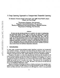
The 10-dimensional data vectors x(t) used in learning are depicted in Fig. 1c. They were generated by nonlinearly mixing the five linear projections of the original sources shown in Fig. 1b, and then adding some Gaussian noise. The standard deviations of the signal and noise are 1 and 0.1, respectively. The nonlinear mixing was carried out using an MLP network having randomly chosen weights and using sinh−1 nonlinearity. The same mixing was used in one of the experiments in [13]. The dimension of the original state space was reduced to five in order to make the problem more challenging. Now the dynamics of the observations is needed to reconstruct the original sources as only five out of eight dimensions are visible instantaneously. The posterior means of the sources of the estimated process after 1,000,000 sweeps are shown in Fig. 1d together with a predicted continuation. This can be compared with the continuation of the original process in Fig. 1a. Figure 2 shows a three-dimensional plot of the state trajectory of one of the original Lorenz processes (top) and the corresponding plot for the estimated sources of the same process (bottom). Note that the MLP networks modeling f and g could have represented any rotation of the source space. Hence separation of the independent processes results only from the form of the posterior approximation. The quality of the estimate of the underlying process was tested by studying the prediction accuracy for new samples. It should be noted that since the Lorenz processes are chaotic, the best that any method can do is to capture its general long-term behavior - exact numerical prediction is impossible. The proposed approach was compared to nonlinear autoregressive (NAR) model which makes the predictions directly in the observation space: x(t) = h(x(t − 1), . . . , x(t − d)) + n(t).

(12)

The nonlinear mapping h(·) was again modeled by an MLP network, but now standard back-propagation was applied in learning. The best performance was given by an MLP network with 20 inputs and one hidden layer of 30 neurons, and the number of delays was d = 10. The dimension of the inputs to the MLP network h(·) was compressed from 100 to 20 using standard PCA. Figure 3 shows the results, averaged over 100 Monte Carlo simulations. The results of the NSSM are from several different simulations that used different initializations. At each stage, the one with the smallest cost function value was chosen. Low cost function values seem to correlate with good prediction performance even though this would not necessarily have to be so. After the first 7500 sweeps the NSSM method was

roughly comparable with the NAR-based method in predicting the process x(t). The performance improved considerably when learning was continued. The final predictions given by NSSM after 1,000,000 sweeps are excellent up to the time t = 1013 and good up to t = 1022, while the NAR method is quite inaccurate already after t ≥ 1003. Here the prediction started at time t = 1000. We have also experimented with recurrent neural networks, which provide slightly better results than the NAR model but significantly worse than the proposed NSSM method.

45 40 35 30 25 20 15

10 5

15

10

0 −5 −10

−15

−10

5

0

−5

2 1.5 1 0.5 0 −0.5 −1 −1.5 −2 1 0.5 0 −0.5 −1

−2

−1.5

−1

−0.5

0

0.5

1

1.5

Fig. 2. The original sampled Lorenz process (top) and the corresponding three components of the estimated process (bottom).

IV. Discussion The NSSM method is in practice able to learn up to about 15-dimensional latent spaces. This is clearly more than many other methods can handle. Currently learning requires a lot of computer time, taking easily days. Finding means to speed up it is therefore an important future research topic. The block approach presented in [17] has smaller computational complexity, and it could help to reduce the learning time, but we have not yet tried it with a NSSM. The proposed method has several potential applications. In addition to the experiments reported here, essentially the same method has already been successfully

a)

0

200

400

600

800

1000

0

200

400

600

800

1000

0

200

400

600

800

1000

0

200

400

600

800

1000

1200

b)

c)

d)

1200

Fig. 1. a) The eight source signals s(t) of the three original dynamical processes. b) The five linear projections of the sources. c) The 1000 ten dimensional data vectors x(t) generated by mixing the projection b) nonlinearly and adding noise. d) The states of the estimated process (t ≤ 1000) and predicted continuation (t > 1000). They can be compared with the original process and its continuation in a).

0

[7]

10

[8] [9]

−1

10

[10]

NAR 7,500 iter. 30,000 iter. 250,000 iter. 1,000,000 iter.

−2

10 1000

1010

1020

1030

1040

1050

Fig. 3. The average cumulative squared prediction error for the nonlinear autoregressive (NAR) model (solid line with dots) and for our dynamic algorithm with different numbers of sweeps.

[11]

[12]

[13]

[14]

applied to detecting changes in the modeled process in [18] and to analyzing magnetoencephalographic (MEG) signals measured from the human brain in [19].

[15]

Acknowledgments This research has been funded by the European Commission project BLISS, and the Finnish Center of Excellence Programme (2000 - 2005) under the project New Information Processing Principles.

[16]

[17]

References [1] [2]

[3]

[4]

[5]

[6]

S. Haykin, Neural Networks – A Comprehensive Foundation, 2nd ed. Prentice-Hall, 1998. Z. Ghahramani and S. Roweis, “Learning nonlinear dynamical systems using an EM algorithm,” in Advances in Neural Information Processing Systems 11 (M. Kearns, S. Solla, and D. Cohn, eds.), (Cambridge, MA, USA), pp. 599–605, The MIT Press, 1999. S. Roweis and Z. Ghahramani, “An EM algorithm for identification of nonlinear dynamical systems,” in Kalman Filtering and Neural Networks (S. Haykin, ed.). To appear. T. Briegel and V. Tresp, “Fisher scoring and a mixture of modes approach for approximate inference and learning in nonlinear state space models,” in Advances in Neural Information Processing Systems 11 (M. Kearns, S. Solla, and D. Cohn, eds.), (Cambridge, MA, USA), pp. 403–409, The MIT Press, 1999. S. Haykin and J. Principe, “Making sense of a complex world,” IEEE Signal Processing Magazine, vol. 15, no. 3, pp. 66–81, May 1998. G. Hinton and D. van Camp, “Keeping neural networks simple by minimizing the description length of the weights,” in Proc. of the 6th Ann. ACM Conf. on Computational Learning Theory, (Santa Cruz, CA, USA), pp. 5–13, 1993.

[18]

[19]

H. Lappalainen and J. Miskin, “Ensemble learning,” in Advances in Independent Component Analysis (M. Girolami, ed.), pp. 75–92, Berlin: Springer, 2000. A. Hyv¨ arinen, J. Karhunen, and E. Oja, Independent Component Analysis. J. Wiley, 2001. H. Attias, “ICA, graphical models and variational methods,” in Independent Component Analysis: Principles and Practice (S. Roberts and R. Everson, eds.), pp. 95–112, Cambridge University Press, 2001. J. Miskin and D. MacKay, “Ensemble Learning for blind source separation,” in Independent Component Analysis: Principles and Practice (S. Roberts and R. Everson, eds.), pp. 209–233, Cambridge University Press, 2001. R. Choudrey and S. Roberts, “Flexible Bayesian independent component analysis for blind source separation,” in Proc. Int. Conf. on Independent Component Analysis and Signal Separation (ICA2001), (San Diego, USA), pp. 90–95, 2001. P. Højen-Sørensen, L. K. Hansen, and O. Winther, “Mean field implementation of Bayesian ICA,” in Proc. Int. Conf. on Independent Component Analysis and Signal Separation (ICA2001), (San Diego, USA), pp. 439–444, 2001. H. Lappalainen and A. Honkela, “Bayesian nonlinear independent component analysis by multi-layer perceptrons,” in Advances in Independent Component Analysis (M. Girolami, ed.), pp. 93–121, Springer-Verlag, 2000. H. Valpola, “Unsupervised learning of nonlinear dynamic state-space models,” Tech. Rep. A59, Lab of Computer and Information Science, Helsinki University of Technology, Finland, 2000. H. Valpola, A. Honkela, and J. Karhunen, “Nonlinear static and dynamic blind source separation using ensemble learning,” in Proc. Int. Joint Conf. on Neural Networks (IJCNN’01), (Washington D.C., USA), pp. 2750–2755, 2001. H. Valpola and J. Karhunen, “An unsupervised ensemble learning method for nonlinear dynamic state-space models,” 2001. Manuscript submitted to Neural Computation. H. Valpola, T. Raiko, and J. Karhunen, “Building blocks for hierarchical latent variable models,” in Proc. Int. Conf. on Independent Component Analysis and Signal Separation (ICA2001), (San Diego, USA), pp. 710–715, 2001. A. Iline, H. Valpola, and E. Oja, “Detecting process state changes by nonlinear blind source separation,” in Proc. Int. Conf. on Independent Component Analysis and Signal Separation (ICA2001), (San Diego, USA), pp. 704–709, 2001. J. S¨ arel¨ a, H. Valpola, R. Vig´ ario, and E. Oja, “Dynamical factor analysis of rhythmic magnetoencephalographic activity,” in Proc. Int. Conf. on Independent Component Analysis and Signal Separation (ICA2001), (San Diego, USA), pp. 451–456, 2001.