International Journal of Sciences: Basic and Applied Research (IJSBAR) ISSN 2307-4531 (Print & Online) http://gssrr.org/index.php?journal=JournalOfBasicAndApplied
--------------------------------------------------------------------------------------------------------------------------------------
Incremental Learning Approach for Enhancing the Performance of Multi-Layer Perceptron for Determining the Stock Trend Basant Ali Sayed Alia*, Abeer Badr El Din Ahmedb, Alaa El Din Muhammad El Ghazalic, Vishal Jain d a
Teaching of Department of Management Information System , Higher Institute of Qualitative Studies, Cairo, Egypt b
c
Lecture of Department Computer Science , Sadat Academy for Management Sciences, Cairo, Egypt
Professor of Department Computer and Information system ,Sadat Academy for Management Sciences, Cairo, Egypt
d
Assistant Professor of Department Computer Applications and Management, Bharati Vidyapeeth's Institute of Computer Applications and Management, New Delhi, INDIA a
[email protected]
b
[email protected]
d
[email protected]
Abstract This paper introduces a new technique for achieving minimum risk of predicting stock trend using multi-layer perceptron. The proposed technique presents the method of classification the stock trend .the paper show a comparison among multi-layer perceptron, gene learning theory. The achieved results show the superior performance of the multi-layer perceptron which is based on mathematical back ground. Keywords:Prediction, Multi-layer Perceptron, Grid search, classification accuracy.
-----------------------------------------------------------------------* Corresponding author. E-mail address:
[email protected]
15
International Journal of Sciences: Basic and Applied Research (IJSBAR)(2014) Volume 16, No 1, pp 15-23
1. Introduction It is sure that the main challenge to discover the technique of Stock market prediction is an applicable and less complicated application of machine learning algorithms. It is found that many various effort in price prediction by using methods such as Neural Network, Linear Regression(LR), Multi Linear Regression(MLR), Auto Regressive Moving Average Models (ARMA) and Genetic Algorithms(GA) .In this report we consider about the Twin Gaussian Process (TGP) method to predict the stock prices. Because of dynamic manner of stock market prices, prediction is so difficult. Increase and decrease of stock market prices depends on various factors such as amount of demand, exchange rate, price of gold, price of oil, political and economic events and … but in the other view point we can consider the stock market price variation as time series and without notation to the mentioned factors, and just by finding the sequence rules of price train, make the price prediction in the future. There are so many researches in price variation time series prediction by different methods such as Neural Network, LR, MLR; ARMA, GA. Neural Network is one of the popular methods for predicating stock market. Most of researches that use Neural Network for prediction, use Multi-Layer Perceptron and use back propagation for learn Network. Who Train Neural Network by historical data of stock for predicting price in future. 2. Limitations of the research • The paper focus on the binary classification process performed by neural network. • The domain of the application is the Egyptian stock market. • The selected sector of the Egyptian stock market is textile sector. • The results achieved under the normal economic conditions of the Egyptian stock market. 3. Adaptive Activation Functions There is a method for improving the performance of the neural network based on enabling the functions of the activation to modify related to the training data characteristics obtained. Using the adaptive activations functions is considered one of the earlier methods which are developed by Zurada. In this case the achieved slope of the selected sigmoid activation function can be learned simultaneously by the achieved weights. In this case the slope parameter λ is gained for every output and hidden layers. Furthermore there is an Additional development is achieved by Engel Brecht et al for the lambda-learning algorithm. Here, the definition of this sigmoid function can be shown as
Such λ is defined as the slope of the function and γ is considered the maximum range. There is an additional development is achieved by Engel Brecht et al for learning equations to can learn the maximum ranges of the used sigmoid functions, thereby doing automatic scaling process which is based on gamma-learning. This development has no need to scale target values to the range (0, 1). The result of modifying the slope and range of the sigmoid function which is called delta learning, the lambda and variations of gamma learning,
16
International Journal of Sciences: Basic and Applied Research (IJSBAR)(2014) Volume 16, No 1, pp 15-23
Fig 1: the Multi-layer perceptron structure 4. Challenges for the Training Multilayer Perceptron Networks The main aim of the training process is discovering the group of weight values that will make the output from the neural network can match the actual target values as closely as possible [2]. No doubt that there are many critical points that involved in designing and training a multilayer perceptron network: • Selecting how many hidden layers to use in the network. •
Deciding how many neurons to use in each hidden layer.
•
Finding a globally optimal solution that avoids local minima.
• Converging to an optimal solution in a reasonable period of time. • Validating the neural network to test for over fitting. 5. Neural network Model Experiments: 4.1. Selective Learning Not much research has been done in selective learning. Hunt and Deller developed Selective Updating, where training starts on an initial candidate training set. Patterns that exhibit a high influence on weights, i.e. patterns that cause the largest changes in weight values [3].are selected from the candidate set and added to the training set. Patterns that have a high influence on weights are selected at each epoch by calculating the effect that patterns have on weight estimates. These calculations are based on matrix perturbation theory[5].Where an input pattern is viewed as a perturbation of previous patterns.If the perturbation is expected to cause large changes to weights, the corresponding pattern is included in the training set. The learning algorithm does use current knowledge to select the next training subset, and training subsets may differ from epoch to epoch [9]. Selective Updating has the drawback of assuming uncorrelated input units, which is often not the case for practical applications. 4.2. Incremental learning
17
International Journal of Sciences: Basic and Applied Research (IJSBAR)(2014) Volume 16, No 1, pp 15-23
Research on incremental learning is more abundant than for selective learning. Most current incremental learning Techniques have their roots in information theory, adapting Fedorov’s optimal experiment design for NN learning[12]. The different information theoretic incremental learning algorithms are very similar, and differ only in whether they consider only bias, only variance, or both bias and variance terms in their selection criteria. One drawback of the incremental learning algorithms summarized above is that they rely on the inversion of an information matrix [7].Fukumizu showed that, in relation to pattern selection to minimize the expected MSE, the Fisher information matrix maybe singular. 4.3. Converging to the Optimal Solution – Conjugate Gradient It is a set of starting weights value where that selected randomly. The suggested approach use the benefits generated from the conjugate gradient technique. Practically, majority of training algorithms are based on similar cycle to select the best values of weights. Firstly, run the values predicted for the case through the selected network based on tentative set of weights [15]. Secondly, calculate the variation among the target predicted and the actual target for the case. This is called the error of the prediction .thirdly; calculate the mean error of the information through the set of training cases. 4. Generate the achieved error backward by the network itself and calculate the gradient (vector of derivatives) of the difference in the achieved error with respect to difference in the values of weight 5 [6]. Perform the current adjustments to the generated weights to reduce the error. Every cycle of this is called a /epoch/. Due to the generated error information is propagated backward by the network, this sort of training technique is called /backward propagation/ or "back prop". The fundamental technique is based on using the /gradient descent/ algorithm to modify the value weights to can convergence based on the gradient [8]. Majority of neural networks use the best of algorithm .this approach can provide the classical conjugate gradient algorithm with line search, but it also offers a newer algorithm, /Scaled Conjugate/ /Gradient/ (see Moller, 1993). This technique is based on using the technique of numerical approximation for the second derivatives that be called Hessian matrix). On the other hand in the same time, it can avoidinstability by combining the model-trust region technique from the Liebenberg-Marquardt technique with the conjugate gradient approach. This permit the scaled conjugate gradient to calculate [3] .what is the optimal step size in the search direction without having to done more expensive computations in line search used by the classical conjugate gradient algorithm. It is sure, that must be a cost involved in evaluating the second derivatives [5]. The performed Tests by Moller show the scaled conjugate gradient algorithm converging up to approximately twice as fast as classical conjugate gradient and up to twenty times as fast as the neural back propagation which is based on gradient descent. Moller's tests also presented that scaled conjugate gradient failed to converge less often than traditional conjugate gradient or back propagation using gradient descent [4]. 4.4. The approach for Avoiding Over fitting Over fitting case “happens only when the parameters of a model are trained so tightly that the model fits the training data well but has poor accuracy on separate data not used for training. Especially the type of network is called Multilayer perceptron's are subject to over fitting as are most other types of models. The paper has a
18
International Journal of Sciences: Basic and Applied Research (IJSBAR)(2014) Volume 16, No 1, pp 15-23
method for dealing with over fitting by selecting the optimal number of neurons. The paper has a method for dealing with over fitting: (1) by selecting the optimal number of neurons as described above, and (2) by evaluating the model as the parameters are being tuned and stopping the tuning when over fitting is detected. This is known as “early stopping”. 6. The proposed algorithm The best neural network structure was chosen from Table (1) below. The selected network has 5 input neurons with 11 hidden neurons and 1 output. Each MLP in Table (1) was trained and tested using different learning rates and epochs. The best network (marked in bold font) was chosen using the least difference between the training and testing data. The motivation for using this criterion is to ensure that the network chosen can predict the stock price as accurate as possible. The proposed algorithm 1- Prepare the data collected. 2- Clean the data. 3- Run the model of neural network optimized by grid search. 4- Compute the relative importance of dimensions. 5- Rank the relative importance of dimensions. 6- Select Best dimensions achieving minimum error. 7- If the minimum errors satisfy acceptable error, stop or else go to step 3. 7. Experiments and results This subsection shows a comparison between neural network and hybrid neural and grid search Input Data Input data file: \csv\bolivar.csv Number of variables (data columns): 47 Data subletting: Use all data rows Number of data rows: 800 Total weight for all rows: 800 Rows with missing target or weight values: 0 Rows with missing predictor values: 1
19
International Journal of Sciences: Basic and Applied Research (IJSBAR)(2014) Volume 16, No 1, pp 15-23
6.1. Neural Network Parameters Number of rows excluded because of missing predictor values = 1 Table1: shows the Neural Network Architecture Layer
Neurons
Activation
Min. Weight
Max. Weight
Input
5
Passthru
Hidden1
13
Linear
-1.483e+000
1.706e+000
Output
3
Linear
-1.787e+000
1.516e+000
Table2: shows Category weights (prior probabilities) Category
Probability
Down
0.5225564
Up
0.4398496
stable
0.0375940
6.1.2. Training Statistics Table3: shows error generated by Conjugate gradient Process
Time
Evaluations
Error
Conjugate gradient
00:00:02.5
806,145
9.5403e-002
6.1.3. Model Size Summary Report Network size evaluation was performed using 4-fold cross-validation. Table 4: shows Network size evaluation was performed using 4-fold cross-validation Hidden layer 1 Neurons
MLP % Misclassifications
IncrementalMLP % Misclassifications
2
42.765433221
37.09273
3
38.67765442
32.20551
4
35.675576
32.83208
5
34.87656578
32.08020
6
34.9876543
32.08020
7
33.86664532
32.58145
8
34.87675445
33.33333
9
34.97776654
31.95489
10
38.677788
34.58647
11
38.8766554
33.83459
20
International Journal of Sciences: Basic and Applied Research (IJSBAR)(2014) Volume 16, No 1, pp 15-23
12
34.678909087
32.08020
13
33.78769