An ensemble of discriminative local subspaces in microarray data for gene ontology annotations predictions. Tomas Puelma, Alvaro Soto Department of Computer Science Pontificia Universidad Cat´olica de Chile
[email protected],
[email protected]
Abstract—Genome sequencing has allowed to know almost every gene of many organisms. However, understanding the functions of most genes is still an open problem. In this paper, we present a novel machine learning method to predict functions of unknown genes in base of gene expression data and Gene Ontology annotations. Most function prediction algorithms developed in the past don’t exploit the discriminative power of supervised learning. In contrast, our method uses this to find discriminative local subspaces that are suitable to perform gene functional prediction. Cross-validation test are done in artificial and real data and compared with a state-ofthe-art method. Preliminary results shows that in overall, our method outperforms the other approach in terms of precision and recall, giving insights in the importance of a good selection of discriminative experiments. Keywords-gene expression; microarray; gene function prediction; feature selection; gene ontology;
I. I NTRODUCTION During the last decades, it has been possible to access the genome sequence of several species, however, understanding the main functions of most genes is still an open problem. In the biological arena is widely accepted that, in general, genes that share some particular function displays similar pattern of expression [1], [3]–[6]. This suggests the idea of predicting unknown gene functions based on the patterns of expression of genes with known biological functions. This approach has been followed by several previous works [9], [11], [13], [19], [20]. Furthermore, gene expression data has also been enriched with additional data sources, such as protein interactions and phenotype information, among others [8]. In terms of known genes functions, the Gene Ontology (GO) project is a major bioinformatics initiative with the aim of standardizing the representation of gene attributes across species and databases [2]. The GO project has developed three structured controlled vocabularies (ontologies) that describe gene products in terms of their associated biological processes, cellular components, and molecular functions in a species-independent manner. In particular, GO annotations are highly structured by biological process terms with a hierarchical ordering from highly general to more specific gene functions.
Rodrigo Gutierrez Department of Molecular Genetics and Microbiology Pontificia Universidad Cat´olica de Chile
[email protected]
In this paper, we use GO terms annotations for genes of Arabidopsis thaliana, a model organism in plant biology. Our goal is to use these known gene functions to predict the functions of unknown genes by comparing their gene expression data. To achieve this, we use the expression of 22 thousand genes under 1701 experimental conditions available from public quality-screened microarray data. Several previous works [9], [11]–[13], [17], [19], [20] have proposed classification schemes to predict gene functions using microarray data and GO terms. In general, most of these works can be classified under two major approaches. On one hand, discriminative approaches based on supervised algorithms that make use of all the available experimental conditions to establish relations among genes. On other hand, unsupervised schemes based on the so-called biclustering approach that search for subspaces of selective experimental conditions to establish meaningful relations between genes. The main contribution of our work resides in proposing a new algorithm that takes advantage of the discriminative power of supervised learning, while at the same time explicitly searching for relations among genes in selective subspaces. Our approach is based on an adaptive nearest neighbor scheme that for each gene with a known function establishes a suitable discriminative subspace to perform gene function prediction. This paper is organized as follows. Section II shows the current state-of-the-art and the main differences with our work. Section III discusses the details of our approach. Section IV shows the results of applying our methodology to the case of synthetic and real datasets. Finally, Section V presents the main conclusions of this work. II. R ELATED W ORK Gene function prediction has been a very active topic in the last decade in the bioinformatics field. Eisen [6] was one of the pioneers in analyzing systematically this kind of data. In his work, he used an average-linkage approach to cluster the budding yeast genes that were co-expressed, using the Pearson correlation coefficient (PCC) as the similarity metric. Interestingly, the clusters grouped genes with known
similar functions, leading to the idea of propagating putative functions to the uncharacterized clustered genes. Many other works have used this co-expression idea to try to predict gene function [9], [11]–[13], [17], [19], [20]. In a recent work, Van de Peer et al. [20] developed a method that predicts function based in the enrichment of GO terms in the gene’s co-expression neighborhood. This is done by calculating the expression similarities between pairs of genes, using the PCC statistic, and then linking the genes with a PCC higher than a given threshold. The neighborhood of a gene is then determined by the genes linked to it. The statistical significance of the enrichment of each GO term in the gene’s neighborhood is evaluated using the hypergeometric distribution, assigning the terms with a 𝑝 − 𝑣𝑎𝑙𝑢𝑒 < 0.05. They applied this method in 129 A. thaliana microarray experiments, but obtained overall low recalls (13 − 34%). In our work we try to improve this, mainly by using the current functional information, to guide the selection of subsets of experiments where the genes of the same functional category may correlate better. In terms of a pattern recognition problem, this can be seen as a feature selection to improve the similarity of the samples of the same class. The idea that the gene’s co-expression patterns may be hidden in a subset of experimental conditions is not new and lots of biclustering algorithms has been developed recently to try to tackle this (See [14], [15], [18] for reviews of biclustering algorithms). In few words, these methods try to find biclusters, that can be defined as a subset of genes that shows co-expression in a subset of conditions. As a clustering algorithm, this search is done in an unsupervised manner. Thus, to classify new data, an enrichment approach like the one used in [17] or [20] is usually done. However, biologically it is expected that genes with different functions can cooperate or function synchronically in some conditions. Thus, one drawback of the biclustering algorithms is that they can find very general subsets of conditions where genes with different functional roles can be co-expressed. This is specially important considering the great amount and diverse nature of the expression data that is being used and that is continually increasing. Our approach tries to overcome this by doing a supervised search of subsets of conditions (features) that maximize the similarity of genes (samples) of the same function (class) and that at the same time minimize the similarity between the genes with different functions (classes). These are key elements that distinguish our method for the current state-of-the-art. III. P ROPOSED M ETHOD In this section we present DLS, our approach for gene function prediction. We start by describing and defining some important characteristics of the problem. Then, we describe the main steps of our algorithm.
A. Problem Definition Gene function prediction based on microarray data and GO annotations can be cast as a machine learning based classification problem. As shown in Table I, we have 𝑁 samples, {𝑆1 , 𝑆2 , . . . , 𝑆𝑁 }, corresponding to 𝑁 genes of a given organism, whose 𝑀 features, {𝐹1 , 𝐹2 , . . . , 𝐹𝑀 }, correspond to their expression levels, measured by microarrays under different experimental conditions. So, we have a data matrix 𝐷𝑎𝑡𝑎𝑀 𝑎𝑡𝑟𝑖𝑥 of 𝑁 × 𝑀 , where 𝐷𝑎𝑡𝑎𝑀 𝑎𝑡𝑟𝑖𝑥(𝑖, 𝑗) holds the expression value of gene 𝑖 under experimental condition 𝑗. Each sample belongs to one or more labels or classes {𝑇1 , 𝑇2 , . . . , 𝑇𝑁 𝑐 } that correspond to the respective GO terms annotations. From now on, we will refer to samples and genes, features and experimental conditions, and classes and GO terms, interchangeably. One relevant property of this type of data is that each sample might belong to multiple classes, as genes can play multiple roles in an organism. To deal with this, we adopted a divide-and-conquer strategy by training a different classifier to each class. In this way, the 𝑁 𝑐 classes problem is decomposed as 𝑁 𝑐 binary class problems. For each classification problem the goal is to predict if a new gene can be assigned to a specific functional annotation of interest, based on a training set of genes that have and don’t have the given function. From now on, we will refer to the target class samples as 𝑐𝑙𝑎𝑠𝑠1 samples, and to the samples that are not from the class as 𝑐𝑙𝑎𝑠𝑠0 samples. Another important characteristic is that not all the genes of the same functional category will necessarily share the same expression patterns in the same conditions. Moreover, GO terms are organized hierarchically, so many, more specific functions are embedded within each term, meaning that there can be subclasses within a class. Hence, we focus in finding discriminant local subspaces (DLS) within the genes of the same function. The idea is for each DLS to represent a discriminative pattern found within the 𝑐𝑙𝑎𝑠𝑠1 samples, so that they can be used to classify new instances. Formally, a DLS can be defined as a two-tuple (𝑆𝐷𝐿𝑆 , 𝐵𝐷𝐿𝑆 ). Here, 𝑆𝐷𝐿𝑆 ∈ 𝑆1 , 𝑆2 , ..., 𝑆𝑁 is a 𝑐𝑙𝑎𝑠𝑠1 training sample and 𝐵𝐷𝐿𝑆 ∈ Λ𝑁 is a binary vector that defines the feature subset where 𝑆𝐷𝐿𝑆 is discriminative. Λ𝑁 is the set of all M Table I G ENE EXPRESSION DATA MATRIX REPRESENTATION USED FOR FUNCTION PREDICTION .
dimensional binary vectors, excluding the null binary vector. The main idea of the algorithm is to find a set of DLS that have a high enough correlation with a subset of the known 𝑐𝑙𝑎𝑠𝑠1 samples, but at the same time to have a sufficiently low correlation with the known 𝑐𝑙𝑎𝑠𝑠0 samples, so that they can be distinguished by it, based in their correlations. B. The Main Algorithm The method can be divided into three main steps: First we present the intuition behind each step, followed by a detailed explanation is given in the next sections. Lets emphasize that we are trying to find embedded patterns within subsets of features, that can discriminate the 𝑐𝑙𝑎𝑠𝑠1 samples from the 𝑐𝑙𝑎𝑠𝑠0 samples (see figure 2 in section IV). Thus, the method starts by selecting an initial subset of features for each 𝑐𝑙𝑎𝑠𝑠1 sample of the training data. Selecting the best (most discriminative) subset of features for each 𝑐𝑙𝑎𝑠𝑠1 sample, in a M dimensional space, requires evaluating 2𝑀 − 1 combinations for each training sample. Searching this huge space exhaustively is unpractical. In our case, we adopted an evolutionary search approach. Genetic Algorithms (GA) ( [7], [16]) are known for their ability to efficiently find near-optimal global solutions in large hypothesis spaces. We tested sequential approaches to do this, but these kind of greedy techniques tend to fall in local optimums. Furthermore, if a forward selection is used, poorly significant correlations are obtained when few characteristics have been selected. On the other hand, backward selection suffers from the high dimensional calculations it must do at the beginning, when the majority of features are selected. In contrast, the GA can directly search a sufficiently small but significant number of features, that can serve as an initial, first approximation to the global optimum. In the second step, the ensemble of DLSs that will define the final classifier is determined. With the GA step, we obtained a seed of selected features for each sample. Now, the objective is to decide which of them will be used as DLSs and to refine the subset of features of each. The DLSs can be seen as experts, whose criterion serves to distinguish certain type of 𝑐𝑙𝑎𝑠𝑠1 samples from the 𝑐𝑙𝑎𝑠𝑠0 samples. In this way, this step is the process to discover potentially good experts, and forming their criterion. Each DLS is created iteratively, by searching the most discriminative 𝑐𝑙𝑎𝑠𝑠1 training sample (𝑆𝐷𝐿𝑆 ) and refining its subset of features (𝐵𝐷𝐿𝑆 ) in a greedy way, so that its discrimination power is maximized. Then, a neighborhood of the DLS is defined, searching for similar 𝑐𝑙𝑎𝑠𝑠1 samples. These are then excluded as potential DLS samples for the future steps, in order to find samples containing different patterns. Each DLS should be able to classify a subset of the samples of the class. Thus, the final classifier is an ensemble of the (weak) classifiers made by each DLS. The third global step of the method is the classification
itself, using the ensemble created and trained in the previous steps to classify new instances. Here, each DLS or expert gives a score between 0 and 1 to each new instance, that is proportional to its confidence in that the new sample is from the class. As each DLS represents a portion of the 𝑐𝑙𝑎𝑠𝑠1 samples, the output of the global classifier is the maximum confidence score given to each sample by a DLSs. The following sections provide a detailed explanation of each of the three mentioned steps. C. GA Feature Selection In this section we provide the main details behind the implementation of the genetic algorithm for feature selection in the context of our problem. For more general details about GA’s see [7], [16]. As we mentioned, the purpose of this GA is to provide an initial seed of discriminative features for each training 𝑐𝑙𝑎𝑠𝑠1 sample. So, the GA receives as input: the 𝐷𝑎𝑡𝑎𝑀 𝑎𝑡𝑟𝑖𝑥, the target 𝑐𝑙𝑎𝑠𝑠1 sample index (𝑆𝑡 ) for which features will be selected, the number of features to select and other GA related parameters (table II). Let’s start by defining the key elements that compose a GA: 1) Hypothesis space (chromosomes and genes). 2) Fitness function and selection method. 3) Crossover mechanism. 4) Mutation mechanism. 5) Population update policy. Hypothesis Space: Each hypothesis or chromosomes represents a set of feature indexes. More formally, each chromosome 𝐻𝑖 , 𝑖 = 1, 2, . . . , 𝑃 , is a subset of fixed length m of the M features, i.e. 𝐻𝑖 ∈ {1, 2, . . . , 𝑀 }, ∣𝐻𝑖 ∣ = 𝑚, where P is the number of chromosomes or population size. Fitness Function and Selection Method: The fitness function should provide higher scores to the hypotheses whose features gives higher correlations between 𝑆𝑡 and his neighboring 𝑐𝑙𝑎𝑠𝑠1 samples and lower correlations between 𝑆𝑡 and his neighboring 𝑐𝑙𝑎𝑠𝑠0 samples. Therefore, the fitness score of a given chromosome is calculated as
𝐹 𝑖𝑡𝑛𝑒𝑠𝑠 =
𝑘 ∑
{𝑆𝑜𝑟𝑡𝑒𝑑𝐶𝑜𝑟𝑟𝑠1(𝑗) − 𝑆𝑜𝑟𝑡𝑒𝑑𝐶𝑜𝑟𝑟𝑠0(𝑗)} , (1)
𝑗=1
where 𝑆𝑜𝑟𝑡𝑒𝑑𝐶𝑜𝑟𝑟𝑠1 and 𝑆𝑜𝑟𝑡𝑒𝑑𝐶𝑜𝑟𝑟𝑠0 correspond to vectors holding the Pearson Correlation Coefficient between the target sample and each 𝑐𝑙𝑎𝑠𝑠1 and 𝑐𝑙𝑎𝑠𝑠0 samples respectively, sorted in a descending order. As can be seen, only the k higher correlations of each class are used in the fitness function. The selection of the hypotheses for crossover and direct transition to the next generation is performed by a probabilistic scheme, by selecting one chromosome at a time, with replacement. In each selection, each chromosome 𝐻𝑖 has a probability 𝑃 𝑟(𝐻𝑖 ) of being selected, with:
𝐹 𝑖𝑡𝑛𝑒𝑠𝑠(𝐻𝑖 ) 𝑃 𝑟(𝐻𝑖 ) = ∑𝑃 , 𝑗=1 𝐹 𝑖𝑡𝑛𝑒𝑠𝑠(𝑗)
(2)
where 𝐹 𝑖𝑡𝑛𝑒𝑠𝑠(𝐻𝑖 ) is the fitness score (equation 1) of the i-est chromosome. Crossover Mechanism: Crossover generates new hypothesis by combining two parent hypothesis from the current population. The idea behind crossover is to generate a diverse offspring in order to search the hypothesis space globally. To do this, first each parent is randomly permuted. Then, the first half of the first parent is transmitted to the new chromosome. All the feature already transmitted are discarded from the second parent, to ensure that no repeated indexes can be transmitted. Finally, the first m/2 indexes that are left in the second parent are selected and transmitted to the new chromosome. This process is repeated, but switching the parents in order to generate a second child chromosome. Mutation Mechanism: Mutation mechanism provides small random perturbations in the chromosomes, in order to explore the hypothesis space locally. To do this, Nm feature indexes are randomly selected from the target chromosome. These are then swapped with other Nm feature indexes, selected randomly from a pool with the entire set of feature indexes, but without the ones currently selected in the chromosome. Nm is initially set to 4. Population Update: Each new population is generated as follows. First, 5% of the population chromosomes with highest fitness are added directly to the next generation. This is done in order to preserve the best solutions. Also, a chromosome with the m most common features in the current population is kept. The idea behind this can be thought as following the wisdom of the crowd. Next, a Pc% of the population is selected using the selection method described before, and submitted to crossover. The offspring of this process is then added to the new population. The remaining 100 − 5 − 𝑃 𝑐% is again selected probabilistically and added directly to the new population. Finally, a Pm% of the new population is submitted to mutation, and with this, the new generation is settled. This process is repeated during Ng generations (iterations). To optimize the algorithm, some parameters are refined during the process. Once the 𝑁 𝑔/2 generation is reached, the crossover population percentage, Pc, is updated to 𝑃 𝑐/2 and the number of mutations per chromosome, Nm, is updated to 𝑁 𝑚/2. Also, once the 3𝑁 𝑔/4 generation is reached, Nm is again updated to 𝑁 𝑚/2. The idea behind this is to increase global search during the first iterations, when the hypothesis are probably far from the optimum, and increase local search as iterations move to interesting areas of the hypothesis space, where more subtle changes are needed. D. DLS Ensemble Creation
Input: 𝑆𝑐𝑙𝑎𝑠𝑠1: The 𝑐𝑙𝑎𝑠𝑠1 training samples. 𝑆𝑐𝑙𝑎𝑠𝑠0: The 𝑐𝑙𝑎𝑠𝑠0 training samples. 𝐹 𝑠𝑒𝑒𝑑: the feature indexes used as initial seed. Output: 𝐷𝐿𝑆𝑠: the set of DLS’s {𝐷𝐿𝑆1 , 𝐷𝐿𝑆2 , ..., 𝐷𝐿𝑆𝑖 , ..., 𝐷𝐿𝑆𝑛 }, where 𝑛 is the number of DLSs found. 1: 𝑆𝑙𝑒𝑓 𝑡 ← indexes of all the 𝑐𝑙𝑎𝑠𝑠1 samples. 2: 𝑖 ← 1. 3: repeat 4: 𝑆𝐷𝐿𝑆,𝑖 ← Use the corresponding 𝐹 𝑠𝑒𝑒𝑑 features to select the most discriminative sample from 𝑆𝑙𝑒𝑓 𝑡. 5: 𝐵𝐷𝐿𝑆,𝑖 ← Refine the set of features of 𝑆𝐷𝐿𝑆,𝑖 using a Stepwise Selection method starting with the features in 𝐹 𝑠𝑒𝑒𝑑(𝑆𝐷𝐿𝑆,𝑖 ). 6: 𝐷𝐿𝑆𝑖 ← (𝑆𝐷𝐿𝑆,𝑖 , 𝐵𝐷𝐿𝑆,𝑖 ) 7: 𝐶𝑜𝑟𝑟𝑠1 ← Compute the correlations between 𝑆𝐷𝐿𝑆,𝑖 and each 𝑐𝑙𝑎𝑠𝑠1 sample in the subspace defined by 𝐵𝐷𝐿𝑆,𝑖 . 8: 𝐶𝑜𝑟𝑟𝑠0 ← Compute the correlations between 𝑆𝐷𝐿𝑆,𝑖 and each 𝑐𝑙𝑎𝑠𝑠0 training sample in the subspace defined by 𝐵𝐷𝐿𝑆,𝑖 . 9: 𝐶𝑜𝑟𝑟𝑇 ℎ ← Use 𝑐𝑜𝑟𝑟𝑠1 and 𝑐𝑜𝑟𝑟𝑠0 to select the minimum correlation where the proportion of 𝑐𝑙𝑎𝑠𝑠1 samples above that threshold is at least 0.5 (50%). 10: 𝑆𝑛𝑏𝑜𝑟𝑠 ← Select form 𝑐𝑜𝑟𝑟𝑠1 the 𝑐𝑙𝑎𝑠𝑠1 samples that have correlation above 𝐶𝑜𝑟𝑟𝑇 ℎ. 11: Delete from 𝑆𝑙𝑒𝑓 𝑡 the samples in 𝑆𝑛𝑏𝑜𝑟𝑠. 12: 𝑖 ← +1. 13: until 𝑆𝑙𝑒𝑓 𝑡 is 𝑒𝑚𝑝𝑡𝑦. Figure 1.
Pseudo-code for the DLS ensemble creation.
Now we provide details about the second main part of our method (figure 1). First, a variable (Sleft) is created to hold the remaining potential 𝑐𝑙𝑎𝑠𝑠1 samples that could be selected as a DLS. Initially, all 𝑐𝑙𝑎𝑠𝑠1 samples are available, so all its indexes are assigned to Sleft. Then, the discrimination power of each 𝑐𝑙𝑎𝑠𝑠1 sample is evaluated, in his corresponding seed of features, and the most discriminative is selected as a DLS. The function used to evaluate the discrimination of each sample is similar, but not equal, to the fitness function used in the GA. The main difference is that now the number of neighbors is important, because it is desired for the potential sample to have the greatest number of 𝑐𝑙𝑎𝑠𝑠1 neighboring samples. Furthermore, we applied a linear transformation to the correlations of the class1 and class0 samples in order to have maximum discrimination in the ranges that are expected. Thus, the designed function to evaluate a sample is ∑𝑛𝑡1 𝑆𝑐𝑜𝑟𝑒 = 𝑚𝑖𝑛𝑀 𝑎𝑥(𝑐𝑜𝑟𝑟𝑠1(𝑗), 0.7, 1.0) ∑𝑗=1 𝑛𝑡0 − 𝑗=1 𝑚𝑖𝑛𝑀 𝑎𝑥(𝑐𝑜𝑟𝑟𝑠0(𝑗), 0.5, 0.8), (3) where 𝑐𝑜𝑟𝑟𝑠1 and 𝑐𝑜𝑟𝑟𝑠0 are the correlations between the
evaluated sample and the 𝑐𝑙𝑎𝑠𝑠1 and 𝑐𝑙𝑎𝑠𝑠0 samples respectively. The function minMax(X,a,b) linearly transforms the values of vector X that are between a and b to values between 0 and 1. Furthermore, all values below a are given a value of 0 and all value above b are given a value of 1. Once a suitable discriminative sample is found, its seed of features is refined, in order to maximize its discrimination power as much as possible. This is done with a greedy, stepwise feature selection. Since the GA returns a seed of m features and we don’t know if the optimum number of features is lower or greater than m, using forward or backward selection could incorrectly bias the search. Hence, we do not force the algorithm to add or delete features. Instead, the method evaluates each already selected feature for deletion and each unselected features for addition, and the best scoring option is taken. In other words, in each iteration, the algorithm will either add or delete the feature that rises the score the most. For this porpoise we use the scoring function defined in equation 3. With the final set of features (𝐵𝐷𝐿𝑆 ) of the discriminative sample (𝑆𝐷𝐿𝑆 ) selected, a complete DLS is determined. Now, we expect that this DLS will be able to represent a certain kind of pattern shared by some 𝑐𝑙𝑎𝑠𝑠1 samples, that we call its neighborhood. In order to discover DLSs that can represent and discriminate other 𝑐𝑙𝑎𝑠𝑠1 samples, the neighboring samples of the current DLS are eliminated from the possible DLS candidates list (𝑆𝑙𝑒𝑓 𝑡). To decide which 𝑐𝑙𝑎𝑠𝑠1 training samples will be considered as part of the neighborhood, a correlation threshold is determined, so that all the 𝑐𝑙𝑎𝑠𝑠1 samples with a correlation with 𝑆𝐷 𝐿𝑆 above the threshold are considered neighboring genes. This threshold is determined as the minimum correlation needed to get a precision of 0.5 within the neighboring samples. This conservative choice was made because we are aware that in real, complex, noisy data, like the gene expression data, it will be impossible in some cases to avoid having some 𝑐𝑙𝑎𝑠𝑠0 samples with high correlations, and therefore, inside the neighborhood. If we wouldn’t consider this, there could be a huge impact in the size of the neighborhood and we could have a lot of redundant DLSs. Furthermore, as will be seen in the artificial data tests (section IV), this works well even if the neighborhoods are well defined. Finally, once the samples from the cluster are selected and removed from the Sleft variable, the process is repeated (steps 4 to 11 in figure 1) until no samples are left in Sleft to be evaluated. E. Classification Here we give the details of how to use those trained DLSs to classify new instances. As mentioned earlier, each DLS represents a pattern, that can be used to discriminate certain type of 𝑐𝑙𝑎𝑠𝑠1 samples from the 𝑐𝑙𝑎𝑠𝑠0 samples. This discrimination is given in the sense that the DLS has high
correlations with some 𝑐𝑙𝑎𝑠𝑠1 samples but low correlations with the 𝑐𝑙𝑎𝑠𝑠0 samples. Thus, a minimum correlation threshold could be used in order to classify new instances. But, as mentioned earlier, real data is not that simple and it isn’t always clear what correlation threshold to use: setting it too high could translate in a poor recall and setting it too low could translate in a poor precision. Moreover, not all the DLS’s have the same degree of discrimination and, therefore, there should be different degrees of confidence to the classifications they do. So, confidence scores are given to each new instance by each DLS, based on the correlations that the DLS has with the training set and with the new instance. Intuitively, the are two factors that should influence the score. First, the proportion of 𝑐𝑙𝑎𝑠𝑠1 and 𝑐𝑙𝑎𝑠𝑠0 training samples that have correlations with the DLS that are “similar” to the one that has the new sample. The higher is the proportion of 𝑐𝑙𝑎𝑠𝑠1 samples, the higher the score. For example, if a new instance has a correlation of 0.85 with a certain DLS, but there are lots of 𝑐𝑙𝑎𝑠𝑠0 samples with correlations (with the DLS) around 0.8 − 0.9, then there is not enough evidence to say that the new instance is from 𝑐𝑙𝑎𝑠𝑠1, so a low confidence should be given. The second factor that should influence the confidence is how “similar” are the correlations. The closer the 𝑐𝑙𝑎𝑠𝑠1 sample correlations are from the new instance correlation, the better, and the opposite is expected from the 𝑐𝑙𝑎𝑠𝑠0 samples. One natural way to measure this would be to use a window of a fixed width, centered in the correlation of the new instance, and counting the number of 𝑐𝑙𝑎𝑠𝑠1 and 𝑐𝑙𝑎𝑠𝑠0 training samples that have correlations that fall inside the window. Each training sample then would vote with a weight proportional to its distance to the center of the window. Thus, the confidence of the new instance, 𝑆𝑛 𝑒𝑤, could be: 𝑤1 , (4) 𝐶𝑜𝑛𝑓 𝑆𝑐𝑜𝑟𝑒(𝑆𝑛𝑒𝑤 ) = 𝑤0 + 𝑤1 where 𝑤0 𝑤1
= =
𝑛𝑡0 ∑ 𝑖=1 𝑛𝑡1 ∑
𝑤(𝑐𝑜𝑟𝑟𝑠1(𝑖), 𝑐𝑜𝑟𝑟(𝑆𝑛𝑒𝑤 ), 𝑤𝑖𝑑𝑡ℎ) 𝑤(𝑐𝑜𝑟𝑟𝑠1(𝑖), 𝑐𝑜𝑟𝑟(𝑆𝑛𝑒𝑤 ), 𝑤𝑖𝑑𝑡ℎ),
𝑖=1
where 𝑐𝑜𝑟𝑟𝑠1(𝑖) and 𝑐𝑜𝑟𝑟𝑠0(𝑖) hold the correlations of the i-est 𝑐𝑙𝑎𝑠𝑠1 and 𝑐𝑙𝑎𝑠𝑠0 samples with the DLS sample, respectively, 𝑐𝑜𝑟𝑟(𝑆𝑛𝑒𝑤 ) is the correlation of the new instance with the DLS sample, and w is the window function { ∣𝑥 − 𝑦∣, ∣𝑥 − 𝑦∣ ≤ 𝑤𝑖𝑑𝑡ℎ) 𝑤(𝑥, 𝑦, 𝑤𝑖𝑑𝑡ℎ) = (5) 0, ∣𝑥 − 𝑦∣ > 𝑤𝑖𝑑𝑡ℎ. The problem with this score is that the window function is binary, so all the training samples that fall outside the window do not have any influence in the score. Thus, we
Table II PARAMETERS USED IN THE TESTS BY THE DLS ALGORITHM .
Part I Part II
#Features 50 Precision 0.5
#Generations 300 Part III
#Chromosomes 100 Width 0.1
Pc 0.6
Pm 0.5
k 5
decided to use a continuous version of the window function. The idea is for all the training samples to have an influence, but that this influence drops rapidly as the distance of the training samples grows. To capture this, we used a Gaussian kernel function as the w function, defined as ) ( (𝑥 − 𝑦)2 1 √ exp − , (6) 𝑤 = 𝑁 (𝑥, 𝑦, 𝑤𝑖𝑑𝑡ℎ) = 2 𝑤𝑖𝑑𝑡ℎ2 𝑤𝑖𝑑𝑡ℎ 2𝜋 where N(x,y,width) is the value of the normal probability density function, centered in y, with standard deviation width and evaluated in x. So, the Gaussian is centered in the correlation of the new instance, and measures each training sample with a weight that decreases with its distance from the center. The width parameter defines the width of the area in which there will be more influence. We thought that a reasonable width should be 0.1. Now, each DLS uses this confidence score to evaluate each new instance. The final output of the classification algorithm is then the maximum confidence score given to each new instance. This confidence output is much richer for the user than a simply binary output, because it gives information about the credibility of the classification. IV. E XPERIMENTAL R ESULTS AND D ISCUSSION The proposed method was implemented in Matlab and evaluated with synthetic and real data. Given the complex and noisy nature of biological data, the initial stage of evaluation uses a synthetic dataset with known discriminative local subspaces. Also, we are currently doing analysis with real gene expression data and some preliminary results are shown in this section. To compare the performance of our approach, we selected a state-of-the-art method [20], that uses a nearest neighbors enrichment method to predict gene function from an expression network (See section II for more details). From now on, we will refer to this method as the NNE (Nearest Neighbors Enrichment) method. The parameters used (table II) for our method were not exhaustively fine-tuned, but were chosen based on tests performed in synthetic data. We are currently working in some details of the GA implementation, so a more exhaustive tune of the parameters will be done after this process. A. Synthetic Data A synthetic data set was created simulating the expected patterns in the real data (figure 2). To do this, a matrix
Figure 2. Characteristics of the artificial database used for testing. There are 4 biclusters embedded in the matrix, but only biclusters 1, 2 and 3 are discriminative, because, contrarily to bicluster 4, they are embedded only within class1 samples.
of 3060 × 800 random values was created. Of the 3060 samples, the first 60 were chosen to be 𝑐𝑙𝑎𝑠𝑠1 samples, and the next 3000 to be 𝑐𝑙𝑎𝑠𝑠0 samples. The expected pattern are represented by a subspace correlation cluster (bicluster). A big bicluster was created so that its samples had a high internal pairwise correlation within its set of features. Then, four partitions of it were embedded within the matrix. Each partition can be considered as a bicluster by its own (𝐵𝐶1 to 𝐵𝐶4) and they represent the different patterns within the samples. The configuration in which these biclusters were embedded was done so that each 𝑐𝑙𝑎𝑠𝑠1 sample belonged to two bicluster. However, only one of them was made to be discriminative. So, for each sample, there a three kind of features: features that don’t belong to a bicluster, features that belong to a non-discriminative bicluster and features that belong to a discriminative bicluster. The features that are discriminative belong to the biclusters embedded only within 𝑐𝑙𝑎𝑠𝑠1 samples (BC1, BC2 and BC3 in figure 2). Contrarily, the non-discriminative features belong to a big bicluster embedded within both 𝑐𝑙𝑎𝑠𝑠1 and 𝑐𝑙𝑎𝑠𝑠0 samples (BC4 in the figure 2). More specific details of the synthetic data created are shown in figure 2. To construct the bicluster, there are several types of mathematical models [14]. We used a coherent values model to create them, because they are relatively simple to construct and are a good representation of the co-expression patterns expected in real data. In this model each cell of a given bicluster must satisfy the following criteria: 𝑎𝑖,𝑗 = 𝜇 + 𝛼𝑖 + 𝛽𝑗 + 𝑁 (0, 𝜎),
(7)
where 𝜇 is a base common value of the entire bicluster, 𝛼𝑖 is the common value adjustment for row i and 𝛽𝑗 is the common value adjustment for column j. 𝑁 (0, 𝜎) is an
Class1 Samples Confidences
Class0 Samples Confidences
Class0 Test Samples Confidences
Class1 Test Samples Confidences 0
0
25 26 27 28 29 30
500
10
500
1000
1500
2000
40
Sample Index
Sample Index
Sample Index
30
Sample Index
1000
20
47 48 49 50
1500
2000
2500
2500
50
3000
59 60 3000
60 0
0.1
0.2
0.3
0.4
0.5
0.6
Confidence
0.7
0.8
0.9
1
0
0.1 0.2 0.3 0.4 0.5 0.6 0.7 0.8 0.9
1
Confidence
0
0.1
0.2
0.3
0.4
0.5
0.6
Confidence
0.7
0.8
0.9
1
3500
0
0.1 0.2 0.3 0.4 0.5 0.6 0.7 0.8 0.9
1
Confidence
Figure 3. Confidence scores obtained by the 𝑐𝑙𝑎𝑠𝑠1 (left) and 𝑐𝑙𝑎𝑠𝑠0 (right) samples from the DLS ensemble trained with the entire artificial data set.
Figure 4. Confidence scores obtained by the 𝑐𝑙𝑎𝑠𝑠1 (left) and 𝑐𝑙𝑎𝑠𝑠0 (right) held-out test samples from the DLS ensemble trained with the remaining 80% of the artificial data set.
aleatory number produced with a normal distribution with standard deviation 𝜎. This term was added to the standard model to introduce some noise to the clusters and make them more real. Otherwise, the pairwise correlations of each sample of the bicluster would be one. The 𝜎 used was 0.5 and with this, we obtained a bicluster with a minimum correlation of ∼ 0.81, a mean correlation of ∼ 0.85 and a maximum correlation of ∼ 0.88. To test if the algorithm is capable to find the discriminative subspaces we first trained a DLS ensemble with the entire data set and then used it to classify the same data. The ideal result would be for the method to find a few DLSs (close to 3) to represent the class1 samples, and with them, give high confidence scores to the remaining 𝑐𝑙𝑎𝑠𝑠1 samples (samples 1 to 60) and low confidences to the 𝑐𝑙𝑎𝑠𝑠0 samples (samples 61 to 3060). After doing this, the method found 8 DLSs. The maximum confidences given to each 𝑐𝑙𝑎𝑠𝑠1 and 𝑐𝑙𝑎𝑠𝑠0 sample are shown in figure 3. Of the 60 𝑐𝑙𝑎𝑠𝑠1 samples, 49 obtained confidences very close to 1 and none of the 𝑐𝑙𝑎𝑠𝑠0 samples obtained confidences above 0.1, including the first 300 samples that were part of BC4. This shows that the method was robust in finding only subspaces that were discriminative, but that it wasn’t able to find all of them. As can be seen in figure 3, all the samples from BC1 were correctly found. This is the easiest bicluster to find, because it has the biggest number of discriminative features. In fact, 29 of the 30 samples of BC1 were found by the first DLS. Also, 19 of the 20 samples from BC2 (samples 31 to 50) were correctly found by the fourth discovered DLS. The two DLSs discovered before (DLSs two and three) belong to BC2 too, but in some way, they managed to find discriminative subspaces with samples from BC1, giving low scores to the rest of the samples. Something similar happened with the DLSs five to eight, that belong to BC3. This is the most difficult bicluster to find, because only 100
of the 800 features are discriminative and only 10 samples belong to it. From this results it can be seen that the method can find with great precision DLSs. However, when the proportion of discriminative features is too low (like in BC3), we found that the GA has trouble to find a good seed of discriminative features. We are currently working in doing some improvements to this part of the method. Also, it is interesting that the method found some DLSs from BC2 and BC3 that are very connected with samples from BC1, a pattern that was not explicitly inserted. This means that it is likely to find aleatory correlation patterns and, as they are aleatory, they could be perfectly found between 𝑐𝑙𝑎𝑠𝑠0 and 𝑐𝑙𝑎𝑠𝑠1 samples, for example, by a biclustering method. This gives more importance to the discriminative nature of the search, in order to avoid those aleatory patterns between 𝑐𝑙𝑎𝑠𝑠0 and 𝑐𝑙𝑎𝑠𝑠1 samples. To test the classification and generalization capabilities of the method, we did a cross-validation test, where a 20% of the samples of each class (1 and 0) were held-out for testing and the remaining 80% was used for training. In this process we were careful to select a 20% of each bicluster for the test set, because a random approach could have not selected any samples from some bicluster or, although improvably, all of them from another. The results obtained in the 𝑐𝑙𝑎𝑠𝑠1 and 𝑐𝑙𝑎𝑠𝑠0 test samples are shown in figure 4. The training results obtained are not shown, but it’s worth mentioning that this time the algorithm found DLSs for all the three biclusters, in spite of the less training samples. This can be seen in the results of the test data (figure 4) in that all the test samples, including the BC3 samples, got high confidence scores. This significant change in the training search can happen due to the stochastic nature of the GA algorithm that this time found a better seed. This also reinforces that further refinements must be made to the GA in order to obtain a better stability and convergence of
the features seeds. In spite of this, the classification in the held-out test samples was perfect, showing the generalization power of the algorithm, that in this case, used only 5 DLSs, corresponding to 5 𝑐𝑙𝑎𝑠𝑠1 samples, to perfectly represent and classify the remaining 𝑐𝑙𝑎𝑠𝑠1 samples. B. Real Data The tests in the artificial data provided good insights about the performance of the method in a controlled environment. However, real gene expression data can be far more complex and thus, cross-validation tests in real data are needed to asses the performance and utility of the method in terms of gene function predictability. The data used for this purpose consists of 20, 858 samples (gene expression profiles) and 773 features (microarray experiments). This data was obtained after the preprocessing of the original microarray data, that consists of 1701 Affymetrix ATH1 microarray slides acquired from the NASC’s International Affymetrix Service (http://affymetrix. arabidopsis.info/). The data was normalized with the RMA method [10] using R’s Bioconductor package and the replicates of the same experiments were averaged, resulting in a final set of 773 microarray experiments (features). Each microarray has 22, 810 probes to measure gene expression. Nevertheless, some probes were filtered out, either because they hybridize to more than one gene or because there is another probe that hybridize the same gene, resulting in a set of 20, 858 unique probe-gene pairs (samples). To be able to do the cross-validation test in this data, we needed to create a gold-standard from the information retrieved from GO. Although the GO database gives information about which genes perform a given function, it doesn’t give certain and explicit information about what genes doesn’t perform that function. In other words, the genes not annotated with a certain term are probably genes that doesn’t perform that function. However, many of them could be genes that it’s still unknown that they perform that function. So, it’s difficult to know which genes to include as 𝑐𝑙𝑎𝑠𝑠0 samples in the gold-standard. If we decided to include all the genes not annotated with a given term as 𝑐𝑙𝑎𝑠𝑠0 samples, then we probably would be including some unknown 𝑐𝑙𝑎𝑠𝑠1 samples as 𝑐𝑙𝑎𝑠𝑠0 samples. The biggest problem is that this ’hidden’ samples could introduce a lot of noise to the method, because they will probably share the correlation patterns from the known 𝑐𝑙𝑎𝑠𝑠1 samples, and therefore, they could hide the discriminative subspaces. So, when constructing the training gold-standard for a term 𝑇𝑘 from GO, we decided to include a gene as a 𝑐𝑙𝑎𝑠𝑠0 sample only if it is not annotated with the term 𝑇𝑘 and if it is annotated with at least one term 𝑇𝑖 , 𝑖 ∕= 𝑘 in which there are no genes annotated with 𝑇𝑘 . The fact that there are no known genes that share the terms 𝑇𝑖 and 𝑇𝑘 gives more confidence in that this functions are not complementary and
Figure 5.
Comparison of the results obtained by DLS and NNE.
in consequence, that the genes participating in the function 𝑇𝑖 will not participate in function 𝑇𝑘 . As a preliminary test of the predictive power of the algorithm, a 10-fold cross-validation test was done in the gold-standard created for the term ’Photosynthesis’ (GO:0015979), that is in the 4th level of the ’Biological Process’ sub-ontology. We used this term for our first analysis because it has been reported [20] that these genes show correlation (co-expression) patterns. Besides, there are 127 genes annotated with this term and 105 of them are in our data set, which is a high enough number to find significant patterns, but low enough to do the tests in a reasonable time. The 𝑐𝑙𝑎𝑠𝑠0 samples were selected with the criteria explained above, resulting in a set of 5342 genes. The NNE method, as a nearest neighbors method, is designed to do a leave-one-out classification. This is, to classify a sample, it uses all the rest of the available samples to determine the nearest neighbors. The total number of 𝑐𝑙𝑎𝑠𝑠1 and 𝑐𝑙𝑎𝑠𝑠0 samples is an important factor in this method, because they can alter the hypergeometric p-value estimation to determine enrichment. So, contrarily to our method, to test the NNE method we used the entire gold-standard set as input, in order to avoid harming its performance. Also, to compute the p-values, we used the number of samples from the gold standard as the total number of samples given to the hypergeometric distribution, as we think is the correct way to do it. Furthermore, we evaluated using the real total number of genes and obtained worst overall results (data not shown). To compare the results of the two methods, a recall vs precision curve (figure 5) was constructed. This is very straightforward in our method, because of its continuous confidence output. To construct the curve we just applied different thresholds to the output and registered the corresponding recalls and precisions. However, the NNE output is binary, so, in order to obtain different grades of recall
and precision, we had to run the method several times with different correlation cutoffs ranging from 0 to 1. As can be seen in figure 5, the results of both methods are far from perfect, but are in fact good results considering the complex nature of the data and that there are almost 50 times more 𝑐𝑙𝑎𝑠𝑠0 samples than 𝑐𝑙𝑎𝑠𝑠1 samples. Comparing both results, it can be seen that our method got better results in almost all the recall and precision space, whose limits are marked in the figure with grey lines. The NNE method got a little better results in the extreme cases, but those are not really very useful. For example, at a recall of 0.1, the NNE and DLS methods got precisions of 1.0 and 0.8 respectively, but at that low recalls is very difficult to predict new genes. In contrast, for example, our method obtained a precision of 0.68 at a recall of 0.52, much better than the precision of 0.40 obtained by the NNE method at the same recall. Despite this, we expected to get a better advantage by using a discriminative subspace approach, specially in terms of recall, because we expect that some patterns will be hidden within subspaces of the data. There are several possible reasons of why we are not achieving this. The first and more obvious is the somewhat mediocre performance of the GA seen in the artificial data. So, this results could get better if we improve the GA mechanism and tune the parameters. Another reason could be for the real data to have very few samples in some clusters, making it very difficult to find a generalizable DLS in each of the 10 folds. In this context, it is important to notice that the NNE method had an advantage in using the leave-one-out strategy compared with the 10-fold cross-validation used to test the DLS method, because it uses all the information to classify each instance and those clusters with few samples are always present. Unfortunately, it is practically impossible to use a leaveone-out strategy with our method, because we would need to train it once for each test sample. Another aspect to mention, is that the similar results obtained by the NNE and the DLS methods in this GO term, could indicate that the genes of the photosynthesis process that share co-expression patterns, do it across a very wide range of experimental conditions, and thus, a subspace approach is not needed to find them. This makes some sense, because photosynthesis is a very global and constitutive process in the plant. Thus, we could get a more marked gain in other more specific processes. Nevertheless, this test demonstrates that the method can do functional predictions that are superior or at least as good as a state-ofthe-art method, and serves to continue our work for further improvements of the method.
to explicitly search for relations among genes in selective subspaces. To our knowledge, this is the only method to date that uses a supervised approach to select discriminative subsets of features in microarray data to predict gene function. The results obtained in real data, although preliminary, shows a significant improvement over a recent work in terms of precision and recall. Although more tests in different GO terms must be done, the results obtained so far are encouraging to continue this direction of work. On one hand, the overall better recall increases our believe in that coexpression patterns can be hidden in a subset of conditions, that regular methods that uses all conditions may be missing. On the other hand, the overall better precisions increases our believe in that the addition of a discriminative selection of subset is important to decrease false positives. The experiments done in the artificial data show that, in most cases, the algorithm accomplishes the task of finding discriminative local subspaces and that they can be used for an accurate prediction. Theoretically, this shows the power of instance based approaches like nearest neighbors when are combined with a good selection of discriminative features. Also, it shows that the global and stochastic search of genetic algorithms and the greedy refinements of sequential feature selection can be a good combination for feature selection. However, the results showed that there’s still room for improvement, as some of the discriminative subspaces couldn’t be found, mainly because the implemented GA wasn’t able to find a good seed of features. We are currently working in improvements for this. One possibility we are evaluating is the addition of a backward selection heuristic before the GA, to discard clearly useless features. This would help to make smaller the huge hypothesis space that must traverse de GA in the search for useful features and may provide a faster and more robust convergence. After this, we expect to have good foundations to train our method with all the currently known functional GO annotations, and be able to predict novel biological functions to genes with vague or no functional GO annotations.
V. C ONCLUSIONS
[1] U. Alon, N. Barkai, D. Notterman, K. Gish, S. Ybarra, D. Mack, and A. Levine. Broad patterns of gene expression revealed by clustering analysis of tumor and normal colon tissues probed by oligonucleotide arrays. Proceedings of the National Academy of Sciences of the United States of America, 96(12):6745–6750, 1999.
In this paper we presented a novel algorithm to enhance the functional prediction of genes in large sets of microarray data. The main contribution of our work resides in taking advantage of the discriminative power of supervised learning
ACKNOWLEDGMENT This work was partially funded by Millennium Science Initiative - MIDEPLAN. We would like to thank Anita Araneda for valuable comments. R EFERENCES
[2] M. Ashburner, C. A. Ball, J. A. Blake, D. Botstein, H. Butler, J. M. Cherry, A. P. Davis, K. Dolinski, S. S. Dwight, J. T. Eppig, M. A. Harris, D. P. Hill, L. Issel-Tarver, A. Kasarskis, S. Lewis, J. C. Matese, J. E. Richardson, M. Ringwald, G. M. Rubin, and G. Sherlock. Gene ontology: tool for the unification of biology. The Gene Ontology Consortium. Nat Genet, 25(1):25–29, May 2000.
[16] M. Srinivas and L. M. Patnaik. Genetic algorithms: A survey. Computer, 27(6):17–26, 1994. [17] A. Tanay, R. Sharan, and R. Shamir. Discovering statistically significant biclusters in gene expression data. Bioinformatics, 18 Suppl 1, 2002.
[3] Sven Bergmann, Jan Ihmels, and Naama Barkai. Similarities and differences in genome-wide expression data of six organisms. PLoS Biol, 2(1):e9, 12 2003.
[18] A. Tanay, R. Sharan, and R. Shamir. Biclustering algorithms: A survey. In In Handbook of Computational Molecular Biology Edited by: Aluru S. Chapman & Hall/CRC Computer and Information Science Series, 2005.
[4] D. Brown, L. Zeef, J. Ellis, R. Goodacre, and S. Turner. Identification of novel genes in arabidopsis involved in secondary cell wall formation using expression profiling and reverse genetics. Plant Cell, 17(8):2281–2295, 2005.
[19] Y. Tao, L. Sam, J. Li, C. Friedman, and Y. Lussier. Information theory applied to the sparse gene ontology annotation network to predict novel gene function. Bioinformatics, 23(13):529–538, 2007.
[5] Joseph L. DeRisi, Vishwanath R. Iyer, and Patrick O. Brown. Exploring the Metabolic and Genetic Control of Gene Expression on a Genomic Scale. Science, 278(5338):680–686, 1997. [6] M. Eisen, P. Spellman, P. Brown, and D. Botstein. Cluster analysis and display of genome-wide expression patterns. Proceedings of the National Academy of Sciences of the United States of America, 95(25):14863–14868, 1998. [7] J. H. Holland. Adaptation in natural and artificial systems. MIT Press, Cambridge, MA, USA, 1992. [8] T. Hughes and F. Roth. A race through the maze of genomic evidence. Genome biology, 9(Suppl 1):S1, 2008. [9] T. Hvidsten, A. Laegreid, and J. Komorowski. Learning rulebased models of biological process from gene expression time profiles using gene ontology. Bioinformatics, 19(9):1116– 1123, 2003. [10] R. Irizarry, B. Hobbs, F. Collin, Y. Beazer-Barclay, K. Antonellis, U. Scherf, and T. Speed. Exploration, normalization, and summaries of high density oligonucleotide array probe level data. Biostat, 4(2):249–264, 2003. [11] J. Bailey-Serres K. Horan, C Jang. Annotating genes of known and unknown function by large-scale coexpression analysis. Plant Physiology, 147(1):41, 2008. [12] WK Kim, C. Krumpelman, and EM Marcotte. Inferring mouse gene functions from genomic-scale data using a combined functional network/classification strategy. Genome Biol, 9(suppl 1):S5, 2008. [13] A. Lagreid, T. Hvidsten, H. Midelfart, J. Komorowski, and A. Sandvik. Predicting gene ontology biological process from temporal gene expression patterns. Genome research, 13(5):965–979, 2003. [14] Sara C. Madeira and Arlindo L. Oliveira. Biclustering algorithms for biological data analysis: A survey. IEEE/ACM Transactions on Computational Biology and Bioinformatics, 1(1):24–45, 2004. [15] Amela Prelic, Stefan Bleuler, Philip Zimmermann, Anja Wille, Peter Buhlmann, Wilhelm Gruissem, Lars Hennig, Lothar Thiele, and Eckart Zitzler. A systematic comparison and evaluation of biclustering methods for gene expression data. Bioinformatics, 22(9):1122–1129, 2006.
[20] K. Vandepoele, M. Quimbaya, T. Casneuf, L. De Veylder, and Y. Van de Peer. Unraveling transcriptional control in arabidopsis using cis-regulatory elements and coexpression networks. Plant Physiol., 150(2):535–546, 2009.