arXiv:0904.0635v6 [stat.CO] 31 May 2010
Approximate Bayesian Computation: a Nonparametric Perspective Michael G.B. Blum CNRS, Laboratoire TIMC-IMAG, Facult´e de m´edecine, 38706 La Tronche Universit´e Joseph Fourier, Grenoble, France Phone: +33 (0)4 56 52 00 65 email:
[email protected]
1
Abstract Approximate Bayesian Computation is a family of likelihood-free inference techniques that are well-suited to models defined in terms of a stochastic generating mechanism. In a nutshell, Approximate Bayesian Computation proceeds by computing summary statistics sobs from the data and simulating summary statistics for different values of the parameter Θ. The posterior distribution is then approximated by an estimator of the conditional density g(Θ|sobs ). In this paper, we derive the asymptotic bias and variance of the standard estimators of the posterior distribution which are based on rejection sampling and linear adjustment. Additionally, we introduce an original estimator of the posterior distribution based on quadratic adjustment and we show that its bias contains a fewer number of terms than the estimator with linear adjustment. Although we find that the estimators with adjustment are not universally superior to the estimator based on rejection sampling, we find that they can achieve better performance when there is a nearly homoscedastic relationship between the summary statistics and the parameter of interest. To make this relationship as homoscedastic as possible, we propose to use transformations of the summary statistics. In different examples borrowed from the population genetics and epidemiological literature, we show the potential of the methods with adjustment and of the transformations of the summary statistics. Supplemental materials containing the details of the proofs are available online.
Keywords: Conditional density estimation, implicit statistical model, simulation-based inference, kernel regression, local polynomial
2
1.
INTRODUCTION
Inference in Bayesian statistics relies on the full posterior distribution defined as g(Θ|D) =
p(D|Θ)π(Θ) p(D)
(1)
where Θ ∈ Rp denotes the vector of parameters and D denotes the observed data. The expression given in (1) depends on the prior distribution π(Θ), the likelihood function p(D|Θ) R and the marginal probability of the data p(D) = Θ p(D|Θ)π(Θ) dΘ. However, when the sta-
tistical model is defined in term of a stochastic generating mechanism, the likelihood can be computationally intractable. Such difficulties typically arise when the generating mechanism involves a high-dimensional variable which is not observed. The likelihood is accordingly expressed as a high-dimensional integral over this missing variable and can be computationally
intractable. Methods of inference in the context of these so-called implicit statistical models have been proposed by Diggle and Gratton (1984) in a frequentist setting. Implicit statistical models can be thought of as a computer generating mechanism that mimics data generation. In the past ten years, interests in implicit statistical models have reappeared in population genetics where Beaumont et al. (2002) gave the name of Approximate Bayesian Computation (ABC) to a family of likelihood-free inference methods. Since its original developments in population genetics (Fu and Li 1997; Tavar´e et al. 1997; Pritchard et al. 1999; Beaumont et al. 2002), ABC has successfully been applied in a large range of scientific fields such as archaeological science (Wilkinson and Tavar´e 2009), ecology (Fran¸cois et al. 2008; Jabot and Chave 2009), epidemiology (Tanaka et al. 2006; Blum and Tran 2008), stereology (Bortot et al. 2007) or in the context of protein networks (Ratmann et al. 2007). Despite the increasing number of ABC applications, theoretical results concerning its properties are still lacking and the present paper contributes to filling this gap. In ABC, inference is no more based on the full posterior distribution g(Θ|D) but on the partial posterior distribution g(Θ|sobs ) where sobs denotes a vector of d-dimensional summary statistics computed from the data D. The partial posterior distribution is defined as (Doksum 3
and Lo 1990) g(Θ|sobs ) =
p(sobs |Θ)π(Θ) . p(sobs )
(2)
Of course, the partial and the full posterior distributions are the same if the summary statistics are sufficient with respect to the parameter Θ. To generate a sample from the partial posterior distribution g(Θ|sobs ), ABC proceeds by simulating n values Θi , i = 1 . . . n from the prior distribution π, and then simulating summary statistics si according to p(s|Θi ). Once the couples (Θi , si ), i = 1 . . . n, have been obtained, the estimation of the partial posterior distribution is a problem of conditional density estimation. Here we will derive the asymptotic bias and variance of a Nadaraya-Watson type estimator (Nadaraya 1964; Watson 1964), of an estimator with linear adjustment proposed by Beaumont et al. (2002), and of an original estimator with quadratic adjustment that we propose. Although replacing the full posterior by the partial one is an approximation crucial in ABC, we will not investigate its consequences here. The reader is referred to Le Cam (1964) and Abril (1994) for theoretical works on the concept of approximate sufficiency; and to Joyce and Marjoram (2008) for a practical method that selects informative summary statistics in ABC. Here, we concentrate on the second type of approximation arising from the discrepancy between the estimated partial posterior distribution and the true partial posterior distribution. In this paper, we investigate the asymptotic bias and variance of the estimators of the posterior distribution g(θ|sobs ) (θ ∈ R) of a one-dimensional coordinate of Θ. Section 2 introduces parameter inference in ABC. Section 3 presents the main theorem concerning the asymptotic bias and variance of the estimators of the partial posterior. To decrease the bias of the different estimators, we propose, in Section 4, to use transformations of the summary statistics. In Section 5, we show some applications of ABC in population genetics and epidemiology .
4
2.
PARAMETER INFERENCE IN ABC
2.1 Smooth rejection In the context of ABC, the Nadaraya-Watson estimator of the partial posterior mean E[Θ|sobs ] can be written as Pn i=1 Θi KB (si − sobs ) m0 = P n i=1 KB (si − sobs )
(3)
where KB (u) = |B|−1K(B −1 u), B is the bandwidth matrix that is assumed to be nonR singular, K is a d-variate kernel such that K(u) du = 1, and |B| denotes the determinant
of B. Typical choices of kernel encompass spherically symmetric kernels K(u) = K1 (kuk), in which kuk denotes the Euclidean norm of u and K1 denotes a one-dimensional kernel. To estimate the partial posterior distribution g(θ|sobs ) of a one-dimensional coordinate of Θ, ˜ that is a symmetric density function on R. Here we will restrict we introduce a kernel K our analysis to univariate density estimation but multivariate density estimation can also be ˜ is denoted b′ (b′ > 0) implemented in the same vein. The bandwidth corresponding to K ′ ˜ ˜ b′ (·) = K(·/b )/b′ . As the bandwidth b′ goes to 0, a simple Taylor and we use the notation K
expansion shows that ˜ b′ (θ′ − θ)|sobs ] ≈ g(θ|sobs ). Eθ′ [K The estimation of the partial posterior distribution g(θ|sobs ) can thus be viewed as a problem ˜ b′ (θi − θ) in equation (3), we obtain of nonparametric regression. After substituting Θi by K the following estimator of g(θ|sobs ) (Rosenblatt 1969) gˆ0 (θ|sobs ) =
Pn
˜
Kb′ (θi − θ)KB (si − i=1 P n i=1 KB (si − sobs )
sobs )
.
(4)
The initial rejection-based ABC estimator consisted of using a kernel K that took 0 or 1 values (Pritchard et al. 1999). This method consisted simply of rejecting the parameter values for which the simulated summary statistics were too different from the observed ones. Estimation with smooth kernels K was proposed by Beaumont et al. (2002).
5
2.2 Regression adjustment Besides introducing smoothing in the ABC algorithm, Beaumont et al. (2002) proposed additionally to adjust the θi ’s to weaken the effect of the discrepancy between si and sobs . In the neighborhood of sobs , they proposed to approximate the conditional expectation of θ given s by m ˆ 1 where
m ˆ 1 (s) = α ˆ + (s − sobs )t βˆ2 for s such that KB (s − sobs ) > 0.
(5)
The estimates α ˆ (α ∈ R) and βˆ (β ∈ Rd ) are found by minimizing the weighted sum of squared residuals
WSSR =
n X
{θi − (α + (si − sobs )t β)}KB (si − sobs ).
(6)
i=1
The least-squares estimate is given by (Ruppert and Wand 1994) ˆ = (X t W X)−1 X t W θ, (α, ˆ β) where W is a diagonal matrix whose ith 1 1 1 s1 − sobs . . X= ··· . 1 s1n − s1obs
(7)
element is KB (si − sobs ), and d d · · · s1 − sobs θ1 .. .. , θ = ... , . . · · · sdn − sdobs θn
and sji denotes the j th component of si . The principle of regression adjustment consists of forming the empirical residuals ǫi = θi − m ˆ 1 (si ), and to adjust the θi by computing
ˆ 1 (sobs ) + ǫi , i = 1, . . . , n. θi∗ = m
(8)
Estimation of g(θ|sobs ) is obtained with the estimator of equation (4) after replacing the θi ’s by the θi∗ ’s. This leads to the estimator proposed by Beaumont et al. (2002, eq. (9))
gˆ1 (θ|sobs ) =
˜ b′ (θ∗ − θ)KB (si − K i i=1 P n i=1 KB (si − sobs )
Pn
6
sobs )
.
(9)
To improve the estimation of the conditional mean, we suggest a slight modification to gˆ1 (θ|sobs ) using a quadratic rather than a linear adjustment. Adjustment with general nonlinear regression models was already proposed by Blum and Fran¸cois (2010) in ABC. The conditional expectation of θ given s is now approximated by m ˆ 2 where
1 m ˆ 2 (s) = α ˘ + (s − sobs )t β˘ + (s − sobs )t γ˘ (s − sobs ) for s such that KB (s − sobs ) > 0. 2
(10)
˘ γ˘ ) ∈ R×Rd ×Rd are found by minimizing the quadratic extension The three estimates (α, ˘ β, 2
of the least square criterion given in (6). Because γ is a symmetric matrix, the inference of γ only requires the lower triangular part and the diagonal of the matrix to be estimated. The solution to this new minimization problem is given by (7) where the design matrix X is now equal to
X =
1 .. .
s11
−
s1obs
···
··· .. .
sd1
− .. .
sdobs
(s11 −s1obs )2 2
(s11
−
.. .
1 s1n − s1obs · · · sdn − sdobs
s1obs )(s21
−
s2obs )
.. .
(s1n −s1obs )2 2
··· .. .
(s1n − s1obs )(s2n − s2obs ) · · ·
(sd1 −sdobs )2 2
.. . (sdn −sdobs )2 2
,
Letting θi∗∗ = m ˆ 2 (sobs ) + (θi − m ˆ 2 (si )), the new estimator of the partial posterior distri-
bution is given by
gˆ2 (θ|sobs ) =
Pn
i=1
˜ ′ (θ∗∗ − θ)KB (si − sobs ) K Pb n i . i=1 KB (si − sobs )
(11)
Estimators with regression adjustment in the same vein as those proposed in equations (9) and (11) have already been proposed by Hyndman et al. (1996) and Hansen (2004) for performing conditional density estimation when d = 1. 3.
ASYMPTOTIC BIAS AND VARIANCE IN ABC
3.1 Main theorem To study the asymptotic bias and variance of the three estimators of the partial posterior distribution gˆj (·|sobs ), j = 0, 1, 2, we assume that the bandwidth matrix is diagonal B = bD. 7
A more general result for non-singular matrix B is given in the Appendix. In practice, the bandwidth matrix B may depend on the simulations, but we will assume in this Section that it has been fixed independently of the simulations. This assumption facilitates the computations and is classical when investigating the asymptotic bias and variance of nonparametric estimators (Ruppert and Wand 1994). The first (resp. second) derivative of a function f with respect the variable x is denoted fx (resp. fxx ). When the derivative is taken with respect to a vector x, fx denotes the gradient of f and fxx denotes the Hessian of f . The variance-covariance matrix of K is assumed to be diagonal and equal to µ2 (K)Id . We also introduce the following notations R R R 2 ˜ = u2 K(u) ˜ ˜ = K ˜ 2 (u) du. Finally, if Xn is a µ2 (K) du, R(K) = K (u) du, and R( K) u u u sequence of random variables and an is a deterministic sequence, the notation Xn = oP (an ) mean that Xn /an converges to zero in probability and Xn = OP (an ) means that the ratio Xn /an stays bounded in the limit in probability. Theorem 1 Assume that B = bD, in which b > 0 is the bandwidth associated to the kernel K, and assume that conditions (A1):(A5) of the Appendix hold. The bias and the variance of the estimators gˆj (·|sobs ), j = 0, 1, 2, are given by 2
E[ˆ gj (θ|sobs ) − g(θ|sobs )] = C1 b′ + C2,j b2 + OP ((b2 + b′2 )2 ) + OP (
Var[ˆ gj (θ|sobs )] =
1 ), j = 0, 1, 2, n|B|
C3 (1 + oP (1)), j = 0, 1, 2, nbd b′
(12)
(13)
with C1 = C2,0 = µ2 (K)
C2,1 = µ2 (K)
˜ θθ (θ|sobs ) µ2 (K)g , 2
gs (θ|s)t|s=sobs D 2 ps (sobs ) p(sobs )
hs (ǫ|s)t|s=sobs D 2 ps (sobs ) p(sobs )
tr(D 2 gss (θ|s)|s=sobs ) + 2
!
,
(14)
! tr(D 2 hss (ǫ|s)|s=sobs ) hǫ (ǫ|sobs )tr(D 2 mss (sobs )) , + − 2 2 (15)
8
C2,2 = µ2 (K)
hs (ǫ|s)t|s=sobs D 2 ps (sobs ) p(sobs )
tr(D 2 hss (ǫ|s)|s=sobs ) + 2
!
,
(16)
and C3 =
˜ R(K)R(K)g(θ|s obs ) . |D|p(sobs )
(17)
Remark 1. Curse of dimensionality The mean square error (MSE) of an estimator is equal to the sum of its squared bias and its variance. With standard algebra, we find that the MSEs of the three estimators gˆj (·|sobs ), j = 0, 1, 2, are minimized when both b and b′ are of the order of n−1/(d+5) . This implies that the minimal MSEs are of the order of n−4/(d+5) . Thus, the rate at which the minimal MSEs converge to 0 decreases importantly as the dimension d of sobs increases. However, we wish to add words of caution since this standard asymptotic argument does not account for the fact that the ‘constants’ C1 , C2 , C3 involved in Theorem 1 also depend on the dimension of the summary statistics. Moreover, in the context of multivariate density estimation, Scott (1992) argued that conclusions arising from the same kind of theoretical arguments were in fact much more pessimistic than the empirical evidence. Finally, because the underlying structure of the summary statistics can typically be of dimension lower than d, dimension reduction techniques, such as neural networks or partial least squares regression, have been proposed (Blum and Fran¸cois 2010; Wegmann et al. 2009). Remark 2. Effective local size and effect of design As shown by equations (13) and (17), the variance of the estimators can be expressed, up to a constant, as
1 g(θ|sobs ) , n ˜ b′
where
the effective local size is n ˜ = n|D|p(sobs )bd . The effective local size is an approximation of the expected number of simulations that fall within the ellipsoid of radii equal to the diagonal elements of D times b. Thus equations (13) and (17) reflect that the variance is penalized by sparser simulations around sobs . Sequential Monte Carlo samplers (Sisson et al. 2007; Beaumont et al. 2009; Toni et al. 2009) precisely aim at adapting the sampling distribution of the parameters, a.k.a. the design, to increase the probability of targeting close to sobs . Likelihood-free MCMC samplers have also been proposed to increase the probability 9
of targeting close to sobs (Marjoram et al. 2003; Sisson and Fan 2010). Remark 3. A closer look at the bias There are two terms in the bias of gˆ0 (·|sobs ) (equation (14)) that are related to the smoothing in the space of the summary statistics. The first term in equation (14) corresponds to the effect of the design and is large when the gradient of Dp(·) is collinear to the gradient of Dg(θ|·). This term reflects that, in the neighborhood of sobs , there will be an excess of points in the direction of Dps (sobs ). Up to a constant, the second term in equation (14) is proportional to tr(D 2 gss (θ|s)|s=sobs ) which is simply the sum of the elementwise product of D and the Hessian gss (θ|s)|s=sobs . This second term shows that the bias is increased when there is more curvature of g(·|s) at sobs and more smoothing. For the estimator gˆ2 (·|sobs ) with quadratic adjustment, the asymptotic bias is the same as the bias of an estimator for which the conditional mean would be known exactly. Results of the same nature were found, for d = 1, by Fan and Yao (1998) when estimating the conditional variance and by Hansen (2004) when estimating the conditional density. Compared to the bias of gˆ2 (·|sobs ), the bias of the estimator with linear adjustment gˆ1 (·|sobs ) contains an additional term depending on the curvature of the conditional mean. 3.2 Bias comparison between the estimators with and without adjustment To investigate the differences between the three estimators, we first assume that the partial posterior distribution of θ can be written as h(θ − m(s)) in which the function h does not depend on s. This amounts to assuming an homoscedastic model in which the conditional distribution of θ given s depends on s only through the conditional mean m(s). If the conditional mean m is linear in s, both C2,1 and C2,2 are null involving that both estimators with regression adjustment have a smaller bias than gˆ0 (·|sobs ). For such ideal models, the bandwidth b of the estimators with regression adjustment can be taken infinitely large so that the variance will be inversely proportional to the total number of simulations n. Still assuming that g(θ|s) = h(θ − m(s)), but with a non-linear m, the constant C2,2 is null so that the estimator gˆ2 (·|sobs ) has the smallest asymptotic MSE. However, for general partial 10
posterior distributions, it is not possible to rank the three different biases. Consequently, when using the estimators with adjustment, the parameterization of the model should be guided toward making the distributions g(θ|s) as homoscedastic as possible. To achieve this objective, we propose, in the next section, to use transformations of the summary statistics. 4.
CHOOSING A REGRESSION MODEL
4.1 Transformations of the summary statistics and the parameters To make the regression as homoscedastic as possible, we propose to transform the summary statistics in equations (5) and (10). Here we consider logarithmic and square root transformations only. We choose the transformations that minimize the weighted sum of squared residuals (WSSR) given in equation (6) in which we take an uniform kernel for the weight function K. The weights KB (si − sobs ) depend on the transformations of the summary statistics and the uniform kernel ensures that the WSSR are comparable for different transformations. Since there are a total of 3d regression models to consider, greedy algorithm can be considered for large values of 3d . Although transformations of the parameter θ in the regression equations (5) and (10) can also stabilize the variance (Box and Cox 1964), we rather use transformations of θ for guaranteeing that the adjusted parameters θi∗ and θi∗∗ lie in the support of the prior distribution (Beaumont et al. 2002). For positive parameters, we use a log transformation before regression adjustment. After adjusting the logarithm of a positive parameter, we return to the original scale using an exponential transformation. Replacing the logarithm by a logit transformation, we consider the same procedure for the parameters for which the support of the prior is a finite interval. 4.2 Choosing an estimator of g(·|sobs ) In Section 3, we find that there is not a ranking of the three estimators gˆj (·|sobs ), j = 0, 1, 2, which is universally valid. Since the three estimators rely on local regressions, of degree 0, 1, and 2, we propose to choose the regression model that minimizes the prediction error of the
11
regression. Because the regression models involve a different number of predictors, we use cross-validation to evaluate the prediction error. We introduce the following leave-one-out estimate CVj =
n X
(m ˆ −i j (si ) − θi ), j = 0, 1, 2,
i=1
where m ˆ −i j (si ) denotes the estimate of m(θi |si ) obtained, in the neighborhood of si , with a local polynomial of degree j by removing the ith point of the training set. 5.
EXAMPLES
5.1 Example 1: A Gaussian model We are interested here in the estimation of the variance parameter σ 2 in a Gaussian sample. Although Approximate Bayesian Computation is not required for such a simple model, this example will highlight the potential importance of the transformations of the summary statistics and of the methods with adjustment. Assume that we observe a sample of size N = 50 in which each individual is a Gaussian random variable of mean µ and variance σ 2 . We assume the following hierarchical prior for µ and σ 2 (Gelman et al. 2003) σ 2 ∼ Invχ2 (d.f. = 1) µ ∼ N (0, σ 2 ),
(18) (19)
where Invχ2 (d.f. = ν) denotes the inverse chi-square distribution with ν degrees of freedom, and N denotes the Gaussian distribution. We consider the empirical mean x¯N and variance s2N as the summary statistics. These two statistics are sufficient with respect to the parameter σ 2 (Gelman et al. 2003). The data come from the well-known Iris data set and consist of the sample of the petal lengths for the virginica species (¯ xN = 5.552, s2N = 0.304, and N = 50). We perform a total of 100 ABC replicates. Each replicate consists of simulating n = 20, 000 Gaussian samples. We consider a spherically symmetric kernel for K and an Epanechnikov kernel for K1 . We assume a diagonal bandwidth matrix B = bD where D contains the standard deviation of each summary statistic in the diagonal and b is the 2.5% quantile
12
of the distances ksi − sobs k, i = 1 · · · n. This procedure amounts to choosing the 500 simulation that provide the best match to the observed summary statistics. In the two following examples, we consider the same number of simulations, the same bandwidth matrix, and the same kernel. Here the true posterior distribution is known exactly (Gelman et al. 2003) and can be compared to the different estimates obtained with ABC. Since σ 2 is a positive parameter, its log is regressed as described in Section 4. As displayed by Figure 1, the estimate with linear adjustment gˆ1 (σ 2 |¯ xN , s2N ) provides a good estimate provided that the empirical variance is log-transformed in the regression setting. The WSSR criterion selects the right transformation here since it is minimum for the logarithmic transformation in all of the 100 test replicates. When considering x¯N and log s2N in the regression, both the linear and the quadratic adjustment provide good estimate of σ 2 by contrast to the method without adjustment (see Figure 1). The cross-validation criterion never selects the method without adjustment, selects 74 times linear adjustment and 26 times quadratic adjustment. 5.2 Example 2: Coalescent model in population genetics ABC was originally developed for inferring parameters of coalescent models in populations genetics (Pritchard et al. 1999). Coalescent models describe, in a probabilistic fashion, the tree-like ancestry of genes represented in a sample. Because the ancestral tree is unknown, the likelihood involves an integral over this high dimensional ancestral tree and is computationally intractable. Here we aim at estimating the Time since the Most Recent Common Ancestor (TMRCA) of a sample of gene. This time is equal to the age of the root of the ancestral tree. A description of the coalescent process and the TMRCA is given in Figure 2. The coalescent prior for the TMRCA and the whole ancestral tree can be described by the following hierarchical procedure 1. Simulate the size of the entire population N according to its prior distribution, a uniform distribution between 0 and 10,000 here. 2. Simulate the Tk ’s, the k th inter-coalescence times, as exponential random variables of
13
B)
50% quantile
97.5% quantile
2.5% quantile
50% quantile
97.5% quantile
1e−01
1e−01
1e+01
1e+01
σ
σ
2
1e+03
2.5% quantile
2
1e+03
A)
Id.
√
Log
Id.
√
Log
Id.
√
Log
No adj. Linear Quadr.
No adj. Linear Quadr.
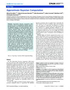
Figure 1: Estimation of the posterior quantiles of the variance parameter σ 2 in a Gaussian sample. We perform a total of 100 ABC replicates and we display the boxplots of the estimated posterior quantiles. A)Estimation of the posterior quantiles with linear adjustment p using (¯ xN , s2N ), (¯ xN , s2N ), and (¯ xN , log s2N ). B) Estimation of the posterior quantiles with
no adjustment and with linear and quadratic adjustment considering (¯ xN , log s2N ) as the summary statistics. The horizontal lines correspond to the true posterior quantiles. In this Gaussian example, both log transformation of the empirical variance and regression adjustment are crucial for accurate estimation of the posterior distribution. Id. stands for the identity function, adj. for adjustment and quadr. for quadratic. rate k(k − 1)/(2N), k = 2 . . . m, where m is the number of sequences in the sample. Time is counted in generations here. The TMRCA is given by the sum of the inter-coalescence times T2 + · · · + Tm . Once the genealogical tree has been generated, DNA sequences are simulated by superimposing mutations along the tree according to a Poisson process of rate u where u is the mutation rate. Here we assume that the mutation rate is known and we use u = 1.8 × 10⁻³ mutation/generation for the whole 500 base pairs DNA sequence (Cox 2008). Assuming the 14
infinitely-many-sites model, each mutation hit a so-called segregating site that has never been hit before. As summary statistics, we consider the total number of segregating sites S and the mean number of mutations between the ancestor and each individual in the sample. The latter summary statistic is called the ρ statistic and is central in the field of molecular dating (Cox 2008).
3
Segregating Number of individuals sites
1 2 6 1
4
TMRCA
A B C D
123456 000100 011000 101000 101011
T2 T3
1 5
2
6
A
B
C
T4
D
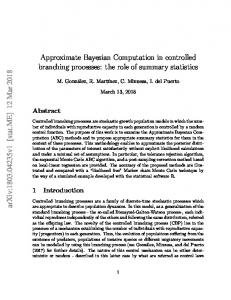
Figure 2: Coalescent process for simulating DNA sequences. This example is excerpted from Cox (2008). There are a total of ten DNA sequences. We display only the upper part of the tree in which mutations occur. We omit the lower part corresponding to the coalescence times T5 , . . . , T10 . The ancestral sequence is a sequence of 500 base pairs and contains a repetition of 0. The stars denote the 0 → 1 mutations. To generate this tree, a mutation rate of 3.6 × 10⁻⁶/base pairs/generation was considered. The true TMRCA is equal to 465 generations here. To infer the TMRCA, we consider the number of segregating sites S = 6 and the mean number of mutations between the ancestor and the individuals ρ = 2.10 as summary statistics. We infer the TMRCA using the DNA sequences simulated by Cox (2008). The true TMRCA was equal to 465 generations in his simulation and the values of the summary statistics are S = 6 and ρ = 2.10. Since the TMRCA is a positive parameter, we use a logarith15
mic transformation when performing the regression adjustment. As shown in Table 1, the WSSR criterion selects the regression equation log TMRCA = log ρ+S. The cross validation criterion points to the estimator with quadratic adjustment although the prediction errors obtained with the linear and quadratic regressions are almost the same (see Table 2). In this example, we do not observe the dramatic effect of the transformations and the adjustments that we found for the Gaussian example. As displayed in Figure 3, both transformations of the summary statistics and regression adjustments do not greatly alter the estimated posterior distribution. Figure 3 also shows that the posterior distribution is clearly more peaky than the prior indicating that the summary statistics convey substantial information about the TMRCA. The 95% credibility interval of the posterior (400 − 2450) is indeed considerably narrower than the credibility interval of the prior (300 − 30, 800). However, as is typical with molecular dating, there remains considerable uncertainty when estimating the TMRCA (Cox 2008). The 95% credibility interval of the TMRCA ranges from a value slightly inferior to the true one to a value more than five times larger than the true one. Table 1: Choosing a transformation of the summary statistics Sum of squared residuals
Parameter TMRCA
ρ+S
Example 2
0.19
Transmission rate α − δ
G+H
Example 3
0.48
R0 = α/δ
G+H
Example 3
1.53
ρ+
√
S
ρ + log S
√ ρ+S
0.18
0.18
0.19 √ G+ H
G + log H
0.48 √
G + log H
G+
√
G+H
√
G+H
0.15 H
1.54
1.33
0.47
√
ρ+
√
S
√
ρ + log S
log ρ + S
0.18 √ √ G+ H
0.18
0.16
√ G + log H
log G + H
0.48 √ √ G+ H
0.15 √ G + log H
log G + H
1.49
1.34
1.51
1.51
0.47
log ρ +
√
S
0.17 log G +
0.17 √
H
log G + log H
√
H
log G + log H
0.48 log G + 1.47
log ρ + log S
0.14
1.34
Table 2: Cross validation criterion for choosing an estimator of the posterior distribution Parameter
No adjustment
Linear adjustment
Quadratic adjustment
TMRCA (Example 2)
0.90
0.624
0.620
Transmission rate α − δ (Example 3)
1.92
0.31
0.34
R0 = α/δ (Example 3)
2.15
1.53
1.65
16
1e−03
No adjustment Linear adjustment Quadratic adjustment
6e−04
8e−04
1e−03
4e−04
6e−04
2e−04
4e−04 2e−04
Density
8e−04
log(ρ) + S ρ+ S ρ+S
0e+00
0e+00
Prior 0
500
1000
1500
2000
2500
3000
0
500
1000
1500
2000
2500
3000
TMRCA
TMRCA (in generations)
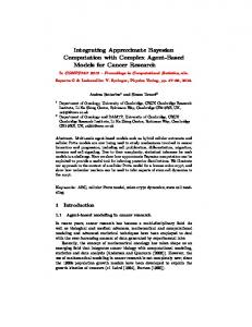
Figure 3: Posterior distribution of the TMRCA. A) Estimated posterior distributions with linear adjustment considering three different transformations of the summary statistics. The summary statistics log ρ and S provide the smallest residual error. B) Estimated posterior distributions using the three different estimates gˆj (TMRCA|(log ρ, S)), j = 0, 1, 2. The quadratic regression provides the smallest prediction error as found with a leave-one-out estimate. For this coalescent example, both transformations of the summary statistics and regression adjustments do not greatly alter the estimated posterior distribution 5.3 Example 3: Birth and death process in epidemiology To study the rate at which tuberculosis spread in a human population, Tanaka et al. (2006) make use of available genetic data of Mycobacterium tuberculosis isolated from different patients. DNA fingerprint at the IS6110 marker were obtained for 473 isolates sampled in San Francisco during 1991 and 1992 (Small et al. 1994). The IS6110 fingerprints were grouped into 326 distinct genotypes whose configuration into clusters is represented by 301 231 151 101 81 52 44 313 220 1282 , where nk indicates there are k clusters of size n. To infer the rate of transmission of the disease from this data, Tanaka et al. (2006) introduced a stochastic model of transmission and mutation. We denote by Xi (t) the number of cases of type i at time t, by G(t) the 17
current number of distinct genotypes, and by N(t) the total number of cases. The model starts with X1 (0) = 1, N(0) = 1 and G(0) = 1. We denote by α, δ, and θ, the per-capita birth rate, death rate and mutation rate. When a birth occurs for an individual of genotype i, the value of Xi (t) is incremented by 1. If the event is a death, the value of Xi (t) is decremented by 1. When a mutation occurs for an individual of genotype i, we assume the infinitely-many-alleles model in which a new allele is formed. This means that the value of Xi (t) is decremented by 1 and a case of a new genotype is created. Following Tanaka et al. (2006), the process is stopped when N = 10, 000. At the stopping time, a sample of size n = 473 is drawn from the final population randomly without replacement. As summary statistics, we consider the total number of genotypes G in the sample and the homozygosity P H of the sample defined as H = (ni /n)2 , where ni , i = 1 . . . G, denotes the number of individual of genotype i in the sample. We consider the following prior specification
θ ∼ N (0.20, 0.072) (
(20)
δ θ α , , ) ∼ Dir(1, 1, 1) | δ < α. α+δ+θ α+δ+θ α+δ+θ
(21)
The informative prior for θ (in mutation/year) arises from previous estimations of the mutation rate (Tanaka et al. 2006). We are interested in the estimation of the net transmission rate α − δ, of the doubling time of the disease log 2/(α − δ), and of the basic reproduction number R0 = α/δ. Since they are positive parameters, they are log-transformed in the regression equations. Once logtransformed, the transmission rate and the doubling time are equal up to a multiplicative constant so that the optimal transformation and adjustment are the same for both parameters. We find that transforming G and H with the log function is optimal for inferring the doubling time whereas log-transforming H only is optimal for inferring R0 (see Table 1). For all parameters, we select linear adjustment based on the cross-validation criterion (see Table 2). As displayed in Figure 4, transformations of the summary statistics and regression adjustments do not greatly alter the estimated posterior distributions except when estimat18
ing R0 . For the transmission rate and the doubling time, the posterior distributions greatly differ from the prior distributions (see Figure 4 and Table 3). However, for the reproduction number R0 , the posterior 95% credibility interval is hardly narrower than the prior credibility interval. These comparisons between the prior and the posterior distributions suggest that the genotype data convey much more information for estimating the transmission rate and the doubling time than for estimating the reproduction number R0 . A large credibility interval for the parameter R0 was also find by Tanaka et al. (2006). Table 3: Posterior estimates of epidemiological quantities for the San Francisco data
a
Parameter
Description
95% Prior C.I.a
Posterior mode
95% Posterior C.I.a
α−δ
Transmission rate (years)
0.01-9.97
0.56
0.16-0.95
log 2/(α − δ)
Doubling time (years)
0.06-57.85
1.16
0.73-4.35
α/δ
Reproduction number R0
1.27-123.32
4.00
2.24-117.45
C.I. stands for credibility intervals
6.
CONCLUSION
In this paper, we presented Approximate Bayesian Computation as a technique of inference that relies on stochastic simulations and non-parametric statistics. We introduced an estimator of g(θ|sobs ) based on quadratic adjustment for which the asymptotic bias involves fewer terms than the asymptotic bias of the estimator with linear adjustment proposed by Beaumont et al. (2002). More generally, we showed that the benefit arising from regression adjustment (equations (9) and (11)) is all the more important that the distribution of the residual ǫ is independent of s in the regression model θ(s) = m(s) + ǫ. To make this regression model as homoscedastic as possible, we proposed to use transformations of the summary statistics when performing regression adjustment. We proposed to select the transformation of the summary statistics that minimizes the sum of squared residuals within the window of the accepted simulations. In a Gaussian example, we showed that transformations 19
0.20
1.2
0.00
0.2 0.0
0.0
0.5
0.05
0.4
0.6
0.10
0.8
0.15
1.0
3.0 1.5 1.0
Density
2.0
2.5
Prior No adjustment Linear adj. + Transf.
0.0
0.5
1.0
Transmission rate
1.5
0.0
0.5
1.0
1.5
2.0
Doubling time
2.5
3.0
0
5
10
15
20
R0
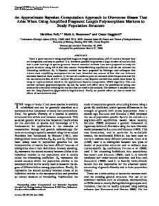
Figure 4: Posterior distributions of key epidemiological quantities for the tuberculosis epidemic in San Francisco. The abbreviation transf. stands for transformation. In this example, both transformations of the summary statistics and regression adjustments do not greatly alter the estimated posterior distributions except when estimating R0 . For the transmission rate and the doubling time, the posterior distributions greatly differ from the prior distributions. For the reproduction number R0 , there is not an important difference between the prior and the posterior indicating than the data do not convey enough information for a confident estimation of R0 . of the summary statistics and regression adjustment can dramatically improve inference in ABC. In two other examples borrowed from the population genetics and epidemiology literature, regression adjustment and transformations of the summary statistics had little effect on the estimated posterior distribution. However, above all, these two examples emphasize the potential of ABC for complex models for which the likelihood is not computationally tractable. APPENDIX APPENDIX A. HYPOTHESES OF THEOREM 1 R A1) The kernel K has a finite second order moment such that uuT K(u) du = µ2 (K)Id
where µ2 (K) 6= 0. We also require that all first-order moments of K vanish, that R is, ui K(u) du = 0 for i = 1, . . . , d. As noted by Ruppert and Wand (1994), this 20
condition is fulfilled by spherically symmetric kernels and product kernels based on symmetric univariate kernels. ˜ is a symmetric univariate kernel with finite second order moment µ2 (K). ˜ A2) The kernel K A3) The observed summary statistics sobs lie in the interior of the support of p. At sobs , all the second order derivatives of the function p exist and are continuous. A4) The point θ is in the support of the partial posterior distribution. At the point (θ, sobs ), all the second order derivatives of the partial posterior g exist and are continuous. The conditional mean of θ, m(s), exists in a neighborhood of sobs and is finite. All its second order derivatives exist and are continuous. A5) The sequence of non-singular bandwidth matrices B and bandwidths b′ is such that 1/(n|B|b′ ), each entry of B t B, and b′ tend to 0 as n− > ∞. APPENDIX B. PROOF OF THEOREM 1 The three estimators of the partial posterior distribution gˆj (·|sobs ), j = 0, 1, 2, are all of the Nadaraya-Watson type. The difficulty in the computation of the bias and the variance of the Nadaraya-Watson estimator comes form the fact that it is a ratio of two random variables. Following Pagan and Ullah (1999, p. 98) or Scott (1992), we linearize the estimators in order to compute their biases and their variances. We write the estimators of the partial posterior distribution gˆj , j = 0, 1, 2, as gˆj (θ|sobs ) = where
gˆj,N , gˆD
j = 0, 1, 2,
n
gˆ0,N =
1X ˜ Kb′ (θi − θ)KB (si − sobs ), n i=1 n
gˆ1,N
1X ˜ = Kb′ (θi∗ − θ)KB (si − sobs ), n i=1 21
n
gˆ2,N = and
1X ˜ Kb′ (θi∗∗ − θ)KB (si − sobs ), n i=1 gˆD =
n X
KB (si − sobs ).
i=1
To compute the asymptotic expansions of the moments of the three estimators, we use the following lemma Lemma 1 For j = 0, 1, 2, we have gˆj (θ|sobs ) =
gj,N ] E[ˆ gj,N ](ˆ gD − E[ˆ gD ]) E[ˆ gj,N ] gˆj,N − E[ˆ + − E[ˆ gD ] E[ˆ gD ] E[ˆ gD ]2 +OP (Cov(ˆ gj,N , gˆD ) + Var[ˆ gD ])
Proof.
(A.1)
Lemma 1 is a simple consequence of the Taylor expansion for the function
(x, y)− > x/y in the neighborhood of the point (E[ˆ gj,N], E[ˆ gD ]) (see Pagan and Ullah (1999) for another proof). The order of the reminder follows from the weak law of large numbers.
The following Lemma gives an asymptotic expansion of all the expressions involved in equation (A.1). Lemma 2 Suppose assumption (A1)-(A5) hold, denote ǫ = θ − m(sobs ), then we have 1 E[ˆ gD ] = p(sobs ) + µ2 (K)tr(BB t pss (sobs )) + o(tr(B t B)), 2
(A.2)
˜ θθ (θ|sobs )p(sobs ) E[ˆ g0,N ] = p(sobs )g(θ|sobs ) + 12 b′2 µ2 (K)g +µ2 (K)[gs (θ|s)t|s=sobs BB t ps (sobs ) + 12 g(θ|sobs )tr(BB t pss (sobs )) + 21 p(sobs )tr(BB t gss (θ|s)|s=sobs )] + o(b′2 ) + o(tr(B t B)),
(A.3)
˜ ǫǫ (ǫ|sobs )p(sobs ) E[ˆ g1,N ] = p(sobs )h(ǫ|sobs ) + 12 b′2 µ2 (K)h +µ2 (K)[hs (ǫ|s)t|s=sobs BB t ps (sobs ) + 21 h(ǫ|sobs )tr(BB t pss (sobs )) + 12 p(sobs )tr(BB t hss (ǫ|s)|s=sobs ) −
hǫ (ǫ|sobs ) tr(BB t mss (sobs ))] 2
+o(b′2 ) + o(tr(B t B)), 22
(A.4)
˜ ǫǫ (ǫ|sobs )p(sobs ) E[ˆ g2,N ] = p(sobs )h(ǫ|sobs ) + 12 b′2 µ2 (K)h +µ2 (K)[hs (ǫ|s)t|s=sobs BB t ps (sobs ) + 21 h(ǫ|sobs )tr(BB t pss (sobs )) + 12 p(sobs )tr(BB t hss (ǫ|s)|s=sobs ) + o(b′2 ) + o(tr(B t B)), V ar[ˆ gD ] = V ar[ˆ gj,N ] =
Proof.
R(K)p(sobs ) 1 tr(BB t ) + O( ) + O( ), n|B| n n|B|
˜ 1 tr(BB t ) b′ R(K)R(K)g(θ|s obs )p(sobs ) +O( )+O( )+O( ), nb′ |B| n nb′ |B| n|B| Cov[ˆ gj,N , gˆD ] =
(A.5)
1 R(K)p(sobs )g(θ|sobs ) + O( ), n|B| n
(A.6) j = 0, 1, 2, (A.7)
j = 0, 1, 2.
(A.8)
See the Supplemental Material available online
Theorem 1 is a particular case of the following theorem that gives the bias and variance of the three estimators of the partial posterior distribution for a general nonsingular bandwidth matrix B. Theorem 2 Assume that B is a non-singular bandwidth matrix and assume that conditions (A1)-(A5) holds, then the bias of gˆj , j = 0, 1, 2, is given by
2
E[ˆ gj (θ|sobs ) − g(θ|sobs )] = D1 b′ + D2,j + OP ((tr(B t B) + b′2 )2 ) + OP (
1 ), j = 0, 1, 2, (A.9) n|B|
with
D1 = C 1 = D2,0 = µ2 (K)
D2,1 = µ2 (K)
gs (θ|s)t|s=sobs BB t ps (sobs ) p(sobs )
hs (ǫ|s)t|s=sobs BB t ps (sobs ) p(sobs )
and D2,2 = µ2 (K)
˜ θθ (θ|sobs ) µ2 (K)g , 2 tr(BB t gss (θ|s)|s=sobs ) + 2
!
,
tr(BB t hss (ǫ|s)|s=sobs ) hǫ (ǫ|sobs )tr(BB t mss ) + − 2 2
hs (ǫ|s)t|s=sobs BB t ps (sobs ) p(sobs )
tr(BB t hss (ǫ|s)|s=sobs ) + 2
The variance of the estimators gˆj , j = 0, 1, 2, is given by 23
!
,
!
,
V ar[ˆ gj (θ|sobs )] =
˜ R(K)R(K)g(θ|s obs ) (1 + oP (1)). ′ p(sobs )n|B|b
(A.10)
Proof. Theorem 2 is a consequence of Lemma 1 and 2. Taking expectations on both sides of equation (A.1), we find that
E[ˆ gj (θ|sobs ]) =
E[ˆ gj,N ] + OP [Cov(gj,N , gˆD ) + Var(ˆ gD )] . E[ˆ gD ]
(A.11)
Using a Taylor expansion, and the equations (A.2)-(A.5), (A.6), and (A.8) given in Lemma 2, we find the bias of the estimators given in equation (A.9). For the computation of the variance, we find from equation (A.1) and (A.11) that
gˆj (θ|sobs ) − E[ˆ gj (θ|sobs )] =
gˆj,N − E[ˆ gj,N ] E[ˆ gj,N ](ˆ gD − E[ˆ gD ]) 1 − + OP ( ). 2 E[ˆ gD ] E[ˆ gD ] n|B|
(A.12)
The order of the reminder follows from equations (A.6) and (A.8). Taking the expectation of the square of equation (A.12), we now find
Var[ˆ gj (θ|sobs ]) =
gj,N ]2 Var[ˆ gD ] E[ˆ gj,N ] 1 Var[ˆ gj,N] E[ˆ + − 2Cov(ˆ g , g ˆ ) + o ( ). (A.13) D j,N P E[ˆ gD ]2 E[ˆ gD ]4 E[ˆ gD ]3 n|B|b′
The variance of the estimators given in equation (A.10) follows from a Taylor expansion that makes use of equations (A.2)-(A.8) given in Lemma 2.
APPENDIX C. SUPPLEMENTAL MATERIALS Proof of Lemma 2 REFERENCES Abril, J. C. (1994), “On the concept of approximate sufficiency,” Pakistan Journal of Statistics, 10, 171–177. 24
Beaumont, M. A., Marin, J.-M., Cornuet, J.-M., and Robert, C. P. (2009), “Adaptivity for ABC algorithms: the ABC-PMC scheme,” Biometrika, 96, 983–990. Beaumont, M. A., Zhang, W., and Balding, D. J. (2002), “Approximate Bayesian computation in population genetics,” Genetics, 162, 2025–2035. Blum, M. G. B., and Fran¸cois, O. (2010), “Non-linear regression models for Approximate Bayesian Computation,” Statistics and Computing, 20, 63–73. Blum, M. G. B., and Tran, V. C. (2008), “HIV with contact-tracing: a case study in Approximate Bayesian Computation, arXiv:0810.0896,”. Bortot, P., Coles, S. G., and Sisson, S. A. (2007), “Inference for stereological extremes,” Journal of the American Statistical Association, 102, 84–92. Box, G. E. P., and Cox, D. R. (1964), “An analysis of transformations,” Journal of the Royal Statistical Society: Series B, 26, 211–246. Cox, M. P. (2008), “Accuracy of molecular dating with the rho statistic: deviations from coalescent expectations under a range of demographic models,” Human Biology, 80, 335– 357. Diggle, P. J., and Gratton, R. J. (1984), “Monte Carlo methods of inference for implicit statistical models,” Journal of the Royal Society: Series B, 46, 193–227. Doksum, K. A., and Lo, A. Y. (1990), “Consistent and robust Bayes procedures for location based on partial information,” Annals of Statistics, 18, 443–453. Fan, J., and Yao, Q. (1998), “Efficient Estimation of Conditional Variance Functions in Stochastic Regression,” Biometrika, 85, 645–660. Fran¸cois, O., Blum, M. G. B., Jakobsson, M., and Rosenberg, N. A. (2008), “Demographic history of european populations of Arabidopsis thaliana.,” PLoS genetics, 4(5).
25
Fu, Y. X., and Li, W. H. (1997), “Estimating the age of the common ancestor of a sample of DNA sequences,” Molecular Biology and Evolution, 14, 195–199. Gelman, A., Carlin, J. B., Stern, H. S., and Rubin, D. B. (2003), Bayesian Data Analysis, Second Edition (Texts in Statistical Science), 2 edn, Boca Raton: Chapman & Hall/CRC. Hansen, B. E. (2004), Nonparametric conditional density estimation,. Working paper available at http://www.ssc.wisc.edu/~bhansen/papers/ncde.pdf. Hyndman, R. J., Bashtannyk, D. M., and Grunwald, G. K. (1996), “Estimating and Visualizing Conditional Densities,” Journal of Computing and Graphical Statistics, 5, 315–336. Jabot, F., and Chave, J. (2009), “Inferring the parameters of the neutral theory of biodiversity using phylogenetic information and implications for tropical forests,” Ecology Letters, 12, 239–248. Joyce, P., and Marjoram, P. (2008), “Approximately sufficient statistics and Bayesian computation,” Statistical Applications in Genetics and Molecular Biology, 7. Article 26. Le Cam, L. (1964), “Sufficiency and approximate sufficiency,” The Annals of Mathematical Statistics, 35, 1419–1455. Marjoram, P., Molitor, J., Plagnol, V., and Tavare, S. (2003), “Markov chain Monte Carlo without likelihoods.,” Proceedings of the National Academy of Sciences of the United States of America, 100, 15324–15328. Nadaraya, E. (1964), “On estimating regression,” Theory of Probability and Applications, 9, 141–142. Pagan, A., and Ullah, A. (1999), Nonparametric econometrics / Adrian Pagan, Aman Ullah, Cambridge, UK: Cambridge University Press.
26
Pritchard, J. K., Seielstad, M. T., Perez-Lezaun, A., and Feldman, M. W. (1999), “Population growth of human Y chromosomes: a study of Y chromosome microsatellites,” Molecular Biology and Evolution, 16, 1791–1798. Ratmann, O., Jørgensen, O., Hinkley, T., Stumpf, M., Richardson, S., and Wiuf, C. (2007), “Using Likelihood-Free Inference to Compare Evolutionary Dynamics of the Protein Networks of H. pylori and P. falciparum,” PLoS Computational Biology, 3, e230. Rosenblatt, M. (1969), “Conditional probability density and regression estimates,” in Multivariate Analysis II, New York: Academic Press, pp. 25–31. Ruppert, D., and Wand, M. P. (1994), “Multivariate locally weighted least squares regression,” Annals of Statistics, 22, 1346–1370. Scott, D. W. (1992), Multivariate density estimation, New York: Wiley. Sisson, S. A., and Fan, Y. (2010), “Likelihood-free Markov chain Monte Carlo,” in Handbook of Markov Chain Monte Carlo, London: Chapman and Hall/CRC Press. Sisson, S. A., Fan, Y., and Tanaka, M. (2007), “Sequential Monte Carlo without likelihoods,” Proceedings of the National Academy of Sciences of the United States of America, 104, 1760–1765. Errata (2009), 106, 16889. Small, P. M., Hopewell, P. C., Singh, S. P., Paz, A., Parsonnet, J., Ruston, D. C., Schecter, G. F., Daley, C. L., and Schoolnik, G. K. (1994), “The epidemiology of tuberculosis in San Francisco: a population-based study using conventional and molecular methods,” New England Journal of Medicine, 330, 1703–1709. Tanaka, M., Francis, A., Luciani, F., and Sisson, S. (2006), “Estimating tuberculosis transmission parameters from genotype data using approximate Bayesian computation,” Genetics, 173, 1511–1520.
27
Tavar´e, S., Balding, D. J., Griffiths, R. C., and Donnelly, P. (1997), “Inferring coalescence times from DNA sequence data,” Genetics, 145, 505–518. Toni, T., Welch, D., Strelkowa, N., Ipsen, A., and Stumpf, M. P. (2009), “Approximate Bayesian computation scheme for parameter inference and model selection in dynamical systems,” Journal of The Royal Society Interface, 6, 187–202. Watson, G. S. (1964), “Smooth regression analysis,” Shankya Series A, 26, 359–372. Wegmann, D., Leuenberger, C., and Excoffier, L. (2009), “Efficient Approximate Bayesian Computation Coupled With Markov Chain Monte Carlo Without Likelihood,” Genetics, 182, 1207–1218. Wilkinson, R. D., and Tavar´e, S. (2009), “Estimating primate divergence times by using conditioned birth-and-death processes,” Theoretical Population Biology, 75, 278–285.
28