Abstract-An equivalent domain integral (EDI) method for calculating J-integrals for two- dimensional cracked elastic bodies is presented. The details of the ...
Engineering Fracture Mechanics Vol. 37, No. 4, pp. 707-725, 1990
Printed in Great Britain.
0013-7944/90 53.00+ 0.00 Pergamon Press plc.
AN EQUIVALENT DOMAIN INTEGRAL METHOD IN THE TWO-DIMENSIONAL ANALYSIS OF MIXED MODE CRACK PROBLEMS I. S. RAJUt
and K. N. SHIVAKUMAR
Analytical Services and Materials, Inc., 107 Research Drive, Hampton, VA 23666, U.S.A. Abstract-An equivalent domain integral (EDI) method for calculating J-integrals for twodimensional cracked elastic bodies is presented. The details of the method and its implementation are presented for isoparametric elements. The total and product integrals consist of the sum of an area or domain integral and line integrals on the crack faces. The line integrals vanish only when the crack faces are traction free and the loading is either pure mode I or pure mode II or a combination of both with only the square-root singular term in the stress field. The ED1 method gave accurate values of the J-integrals for two mode I and two mixed mode problems. Numerical studies showed that domains consisting of one layer of elements are sufficient to obtain accurate J-integral values. Two procedures for separating the individual modes from the domain integrals are presented. The procedure that uses the symmetric and antisymmetric components of the stress and displacement fields to calculate the individual modes gave accurate values of the integrals for all problems analysed. The ED1 method when applied to a problem of an interface crack in two different materials showed that the mode I and mode II components are domain dependent while the total integral is not. This behavior is caused by the presence of the oscillatory part of the singularity in bimaterial crack problems. The ED1 method, thus, shows behavior similar to the virtual crack closure method for bimaterial problems.
NOMENCLATURE half-length or length of crack half-width or width of plate ith domain considered in the domain integral evaluation Young’s modulus of the homogeneous material Young’s moduli of materials 1 and 2 in a bimaterial plate mode I and mode II J-integrals Antisymmetric J and product integrals Symmetric J and product integrals J and product integrals Jacobian matrix of an isoparametric element shape function of the jth node of an isoparametric element normal vector to the contour r component of the normal II in the jth direction remote uniform applied stress or uniform crack face pressure loading S-function defined in eq. (7) displacement in the x,- and x,-directions, respectively antisymmetric components of displacements in the x,- and x,-directions, respectively symmetric components of displacements in the x,- and x,-directions, respectively strain-energy density Cartesian coordinates contours around the crack tip strain tensor Poisson’s ratio of a homogeneous material Poisson’s ratios of materials 1 and 2 of a bimaterial plate stress tensor denotes the transpose of a matrix or column vector
INTRODUCTION STRESS-INTENSITY factors or strain-energy release rates are used to characterize the severity of the stress and strain fields at cracks or delaminations in elastic bodies. Numerous procedures exist in the literature to compute the stress-intensity factors or strain-energy release rates by analytical and tPresent address: Department of Mechanical Engineering, North Carolina A&T State University, Greensboro, NC 27411, U.S.A. EFM
37,4-A
707
I. S. RAJU
708
and K. N. SHIVAKUMAR
numerical methods. For cracks in elastic-plastic materials, the J-integral was proposed[l-31. As originally formulated, the J-integral is a closed contour integral of the strain-energy density and work done by tractions around the crack tip. The J-integral is a path-independent parameter and is equivalent to the rate of change of total potential energy with reference to the crack length. For elastic bodies the J-integral is equivalent to the strain-energy release rate. Although the J-integral is a potential parameter to define the severity of the rack tip in elastic and elastic-plastic materials, it is cumbersome to compute in finite element analyses. Therefore, alternate forms of computing this integral have been proposed[4-111. In refs[6] and[7], procedures based on the virtual crack extension technique[4,5] were proposed to compute the strain-energy release rates (and hence the J-integral). In refs[&lO] line J-integrals were converted to equivalent area or domain integrals, hence the name equivalent domain integral (EDI). The conversion of line integrals to domain integrals is very attractive because all the quantities necessary for computation of the domain integrals are readily available in a finite element analysis. The ED1 method also appears to be a powerful tool to calculate the J-integrals for elastic-plastic materials and problems involving other material nonlinearities. In refs[8-101, the J-integrals were written as area or domain integrals by using the divergence theorem. Closer examination of the integrals shows that the domain integrals are insufficient to satisfy all conditions. The domain integral form of refs[&lO] are valid for the evaluation of the total J-integrals when the crack faces are traction-free and for mixed-mode problems when the stress field around the crack tip contains only the square-root singular terms. However, in a general crack problem, the stress distribution near the crack tip contains both singular and non-singular terms. Thus, the ED1 method needs to be addressed with respect to general mixed-mode problems. The purpose of this paper is to present a detailed formulation of the ED1 method applicable to mixed mode problems under general loading and to study two methods for the separation of modes in mixed mode crack problems. The ED1 method and its numerical implementation in the context of a finite element analysis with isoparametric elements is also presented. The method is then applied to two mode I problems and two mixed mode problems to study the sensitivity of fracture parameters to variables used in the ED1 algorithm and to evaluate the methods for the separation of modes in mixed mode problems.
CONTOUR
AND DOMAIN
INTEGRALS
Consider a crack in a plate subjected to an arbitrary remote loading with an arbitrary closed contour r around the crack tip, as shown in Fig. 1. Then the J-integral is defind in the absence of any body forces as[l-31 r Jr, = Q dr (1) Jr where k = 1, 2 and Q =
Wn,-o,$n, k
(2)
1
e X2
n
0
Xl
I-
(b) Domain bounded by contours rO and r,.
(a) Coordmate system and contour r around the crack tip.
Fig. 1. Contours
around
the crack
tip.
Two-dimensional analysis
709
In eq. (2) W is the total strain-energy density defined as (3) In eqs (2) and (3) rry is the stress tensor, cii is the total strain (which is the sum of the elastic and plastic strains) and nj is the component in thejth direction of the vector II normal to the contour r. The indices i, j and k take the values 1 and 2 for two-dimensional (2D) problems. The X, and x2 represent the directions along the normal to the crack line, respectively. The integrals JX, and Jx2 are two path-independent integrals that define the total amount of the energy flux leaving the contour r in the two directions x, and x2, respectively. J,, is usually termed the J-integral and J,.. is called the product integral. As previously mentioned, the line integrals of eq. (1) are cumbersome to compute in a finite element analysis. In contrast, an area or domain integral is very convenient to compute in a finite element analysis. Therefore, an alternate form of eq. (I), called the equivalent domain integral (EDI), was proposed[8, 10, 111.A more detailed formulation of the ED1 applicable for mixed mode problems and its numerical implementation is presented here. Consider two contours To (OABCO) and r, (ODEFO) around the crack tip as shown in Fig. l(b). The two contours will enclose an area DEFCBAD. By multiplying the integral over r. by unity and the integral over r, by zero, Jxk can be expressed as (4) This manipulation is performed to convert the line intergals into an area or a domain integral. Equation (4) can be expanded as (5) An arbitrary but continuous
function S(x,, x2) is introduced that has the property w,
on r,,,
rDEF.
=
1
x2)
=
0
and W,,
on
9 x2)
Using this S-function,
(6)
eq. (5) can be written as
(7) A closed contour integral along DEFCBAD can be defined easily by adding and subtracting the line integrals on the crack faces FC and AD as
=-
s
Qsdr+S_QSdr+S,,asdr+bQdr+~~AQdr
(8)
Qs dr + were used. In conventional finite element analysis, the equations of equilibrium are not satisfied pointwise in the domain that is modeled. Numerical expe~mentation showed that the differences between including and not including the terms involving the equations of eq~lib~um, are of the order of low3 to 10e4 of the integral values for several problems. Therefore, in writing eq. (12) the equations of equilibrium are assumed to be satisfied exactly. The term in brackets in the second integral in eq. (12) is identically equal to zero pointwise for a linear elastic material. This term, however, is non zero in elastic-plastic problems. Although only linear elastic materials are considered in this report, this term is included because the algo~thm is intended for use with nonlinear material problems. The domain integral in eq, (12) can be rewritten in a form convenient to numerical computation as
(13) where
Two-dimensional analysis
bl=
611Ql2 [ 0120221
{S>T = {EE}. The strain-energy
distribution
711
(14)
W is
w = tbll~ll + =22c22+ 2Q,2Q21.
(1%
The numerical implementation of eq. (13) in a finite-element analysis with isoparametric elements is presented in Appendix A. The integral JX, in eq. (13) for the linear elastic case is equivalent to the strain-energy release rate calculated by the virtual crack extension method since the right hand side of this equation represents the energy change per unit crack extension[8]. Equation (13) is also equivalent to an equation obtained by de Lorenzi[6,7], by calculating the change in energy by mapping a crack configuration with a crack length of a to another crack configuration of length a + da. Line integrals. The four line integrals in eq. (8) are
(J,),,,=~~~Qsdr+S,asdr+S,Qdr.+~~~Qd~.
(16)
When the term Q (defined by eq. 2) is zero on the crack faces, obviously, the line integrals are zero. On the crack faces, n, is always zero; when the crack face is traction free, cl2 and CT~are zero. Thus, for traction-free crack faces, the line integrals in JX, always vanish. This is not the case with Jx2, the product integral. The term Q contains the term Wn,; n2 = - 1 on the line FO and n2 = 1 on the line OD. Thus, even for traction-free crack faces, Q (and line integral in Jx,) can be non-zero. If only mode I deformations exist, then the strain-energy density W is zero on lines FO and OD, and, thus, Q, and the Jx, line integrals are zero for traction-free crack faces. When mode II deformations occur and only the square-root singular term exists in the stress field, the sum of the integrals on FO and OD is zero due to the antisymmetric nature of the deformations, and again the Jx2 line integrals are zero. But in a general crack problem subjected to external loading, both singular and non-singular stress fields exist around the crack tip; thus, the JXZline intergrals will be non-zero (see Appendix B for details). Evaluation of the line JX2intergrals is complicated by the singular stress field and the strain-energy density at the crack tip because of the line integrals on CO and OA. Thus, a method of calculating the mode I and mode II components in mixed mode problems, the decomposition method, in which the Jx2 line integrals vanish is presented in the next section. Separation of modes in mixed mode problems Direct method. The two integrals Jx, and Jx, of eq. (10) can be used to establish the individual modes. If J, and J,, correspond to the pure mode I and pure mode II deformations, then[3, lo]
Jx,= J, + J,, Jx, = - 2&.
(17)
From eq. (17), J, and J,, can be computed in terms of Jx, and Jx, as
JI = tL,/n
+ dml’
J,, = :l,/‘n
- ,/-I’
Jtota, = J, + J,, .
(18)
For general mixed mode deformation the computation of J,., and Jx2 from eq. (13) and the use of eqs (17) and (18) completely define the individual modes. However, for either pure mode I or pure mode II deformations the values of J,, and Jx2 alone are insufhcient to determine the individual modes. (Additional information such as the local crack tip deformation is needed to define the mode.) This is because in either case Jx, = 0 and Jx, gives the total integral. Equation (18) then suggests that only J, exists. This difficulty is due to the choice of the positive sign for the square root terms in eq. (18).
I. S. RAJU and K. N. SHIVAKUMAR
712
t_l.! x2
X1
t2f’S
Svmmetric cbmponents
Antisvmmetric
Symmetric components
Fig. 2. Symmetric and antisymmetric displacement components.
Antisymmetric components
Fig. 3. Symmetric and antisymmetric stress components.
Decomposition method. As previously mentioned, the advantage of transforming the contour integral into a domain integral is lost because of the non-zero line integrals in JX,. These line integrals are necessary to account for the terms containing the product of the singular and non-singular stress (strain) fields in the strain-energy density expression. It is shown in Appendix B that the product terms can be eliminated by decomposing the stress and displacement fields into symmetric and antisymmetric parts. The resulting equation contains only the domain integral. This method termed as the decomposition method is described below. Consider two points P (x1, x2) and P’ (x, , -x2) that are in the immediate neighborhood of the crack tip and are symmetric about the crack line as shown in Fig. 2. For general mixed mode deformations the displacements at P and P’ can be expressed as a combination of symmetric and antisymmetric components as shown in Fig. 2. Then
i:::}
= {:::}
+ {::::}
(19)
and
where subscripts S and AS denote the symmetric and antisymmetric components, respectively. Equations (19) and (20) can be used to determine the symmetric and antisymmetric displacements in terms of the displacements at points P and P’ (see Fig. 2) as
(21) Similarly, the symmetric and antisymmetric components terms of the stresses at points P and P’ (see Fig. 3) as
of the stresses can be expressed in
{~Z}s=;{Z~~}
(22)
Two-dimensional analysis
713
The symmetric and antisymmetric displacements (eq. 21) and stresses (eq. 22) can be used to evaluate the four integrals JsX,, Jsx2, JAsx,, and JAsxzusing eq. (10). Note that the integrals Jsx, and JAsx, (domain and line components individually) will be identically zero because of the symmetric and antisymmetric nature of the stress and displacement fields. The individual modes, J, and Jlr, are now
JI = Jsx, Jn = J~sx, Jtota~ = Jsx,+ JAG, .
(23)
Obviously, this procedure involves an additional step to evaluate the symmetric and antisymmetric components from eqs (21) and (22). However, the individual modes are directly available from the domain integrals Jsx, and JAsx,. For pure mode I problems JAsx, E 0 and J lotal= Jsx,. For pure mode II problems Jsx, = 0 and Jtoutl= JAsx,. Crack -face pressure loading
In the above discussion, the crack faces were assumed to be stress free. When the crack faces are subjected to applied loading, additional terms need to be included in the domain integral formulation. Again consider eq. (10)
(10)
Jxk= (Jx,homain +