phenomena in incompressible fluid flow) using a boundary-domain integral method. A velocity-vorticity formulation of the Navier-Stokes equations is adopted ...
i
Engineering Analysis with Boundary Elements 15 (1995) 359-370 Copyright © 1995 Elsevier Science Limited Printed in Great Britain. All rights reserved 0955-7997/95/$09.50
0955-7997(95)00036-4
ELSEVIER
Boundary-domain integral method using a velocity-vorticity formulation L. Skerget & Z. Rek Faculty of Mechanical Engineering, University of Maribor, Smetanova 17, SI-62000 Maribor, Slovenia
The paper deals with the numerical solution of fluid dynamics (transport phenomena in incompressible fluid flow) using a boundary-domain integral method. A velocity-vorticity formulation of the Navier-Stokes equations is adopted, where the kinematic equation is written in its parabolic version. words: Boundary element method, velocity-vorticity incompressible viscous fluid. Key
formulation,
I INTRODUCTION
2 NAVIER-STOKES EQUATIONS
The Navier-Stokes equations represent a set of highly non-linear partial diffeiential equations for viscous Newtonian fluid motion. They provide a mathematical model of physical consexwation laws of mass, momentum, energy and species concentration. The mathematical formulations may be written for primitive physical or for dependenl variables.l-6 For the selection of the most appropriate formulation it is of great importance which numerical technique is to be applied. In this paper, a boundary-domain integral method is presented for the solution of general fluid motion problems which is based on the velocity-vorticity formulation of the Navier-Stokes equations. The advantages of this approach lie with the numerical separation of kinematic: and kinetic aspects of the fluid flow from the pressure computation, which is determined afterward by solution of a linear system of equations for known velocity and vorticity fields. 7-L° Since the pressure does not appear explicitly in the field equations, the well known difficulty connected with the computation of the pressure boundary values in incompressible fluid flow is avoided. Particular attention is given to formulating appropriate integral representations for all field functions based on the parabolic diffusion equation and on the modified Helmholtz fundamental solution respectively. For the kinematic velocity equation, the false transient approach is applied to increase the convergence rate of the proposed numerical algorithm.
2.1 Primitive variables formulation
The partial differential equation set governing transport phenomena in incompressible fluid motion represents the basic conservation balances of mass, momentum, energy and species concentration written below in an indicial notation form for a right-handed Cartesian coordinate system
(1)
°VJ = o
Dv i PO D--I --
DT p°Cp D---i -
0t7 OTij Ox i ]" ~ "~ Pofi
(2)
Oq/ OXj 4- IT + @
D C = _ Ojj 4- I c Dt Oxi
(3) (4)
where vi is the ith instantaneous velocity component, xi is the ith coordinate, D / D t represents the substantial or Stokes derivative, p is the pressure, 7-ij is the viscous stress tensor and j~ stands for the body force, e.g. the gravity qi. The quantities Po, Cp, IT and Ic are respectively the constant fluid mass density, specific isobaric heat capacity, heat source or sink, and the rate of production or destruction of species by chemical reaction. The variables T, C, qj and J1 stand for temperature, concentration, heat flux and mass flux respectively. The term ¢ is the Rayleigh viscous dissipation function, given by the 359
L. Skerget, Z. Rek
360 expression
'~ = "rij Oxj
(5)
which converts the mechanical energy to the heat acting as an additional heat source. The current discussion will be restricted to the heat radiation transparent fluid, obeying a simple linear gradient type of constitutive hypothesis, namely Newton's, Fourier's and Fick's law, describing respectively the relation between the viscous stress tensor %. and the strain tensor ~ij 7-ij = 2rloeij
(6)
the heat flux vector qj and the temperature field T(rj, t)
OT qJ = --A° ~Xj
(7)
and the mass flux vector jj and the concentration field C(rj, T) OC jj = -aco Oxj (8) where material constants ~/o, Ao and aco are the respective fluid dynamic viscosity, heat conductivity and mass diffusivity. Substituting the above constitutive relations into the basic conservation laws, the nonlinear Navier-Stokes equations set can be derived, expressing the transport phenomena in incompressible Newtonian fluid flow
OVJ=o
where Po is a reference density at temperature To and bT is thermal volume expansion coefficient. The above Navier-Stokes equations set represents a closed parabolic initial boundary value problem for the determination of velocity v;, pressure p, temperature T and concentration C fields. The mathematical description of the transport phenomena in fluid flow is completed by providing suitable Dirichlet, Neuman or Cauchy type boundary conditions, as well as some initial conditions, e.g. for the velocity vector v; Vi
on
F
vi=~io
in
f~ at
Vi =
for
t > to
(15)
t=t o
for the temperature scalar field T T = ~P
on
F 1 for
t > to
qn = (In qn = aT(T - Tf) T=f'o
on
F2
for
t > to
on in
F3 [2
for at
t > to t=t o
(16)
where aT and Tf respectively are the heat transfer coefficient and ambient temperature, while for the scalar concentration field C one may prescribe C= C
jn=~ j.=ac(C-Cf) C=Co
on
F 1
for
t > to
on
F2
for
t>to
on
F3
for
t>to
in
f~
at
t=to
07)
with a c being the mass transfer coefficient and Cf ambient concentration.
(9)
2.2 Velocity-vorticity variables formulation Dv i D---t -
10P 02% Po Ox~ + v° OxjOxj t- Fgi
(10)
DT o~ T IT ¢ 4+-Dt = aTo OxjOxj poCpo poCpo
(11)
DC 02C --4-Ic Dt = ac° OxjOxj
(12)
(13)
where the function F has to be physically justified, e.g. for a number of fluids the following normalized difference density expression can be applied P - Po = F = --/~T(T - To) Po
Ovk
OJi = eijk OXj '
where the quantities aTo = Ao/poCpo, vo = rlo/Po and P = p - pogjrj are respectively the thermal diffusivity, kinematic viscosity and modified pressure. The natural convection effect is considered in the momentum equation by using Boussinesq's approximation, where the temperature influence on fluid mass density is considered only with the body force term f/, while it is neglected in all other terms, where it is assumed to be invariant. The following general expression for density variation can be used p = po(1 + F )
With the vorticity vector oJi representing the curl of the velocity field, e.g. written in symbolic notation
(14)
Owi = 0 OX i
(18)
where e/jk ( i , j , k = 1,2,3) is the permutation unit tensor, that equals 1, if the subscripts /jk are in cyclic order or equals - 1 , when they are in anticyclic order and zero otherwise, the fluid motion computation scheme is partitioned into its kinematic and kinetic aspect) ° The kinetics are governed by the vorticity transport equation obtained as a curl of the momentum eqn (10), rendering the statement
D¢oi Oo~jvi 02~i OF Dt = Oxj + Vo OxjOxy F e i j k g k -@Xj
(19)
describing the redistribution of the vorticity vector in the fluid flow field. Equation (19) shows that the rate of change of the vorticity as one follows a fluid particle, given by the Stokes deviation on the left hand side of the equation, is due to the vortex stretching and twisting, viscous diffusion and buoyancy effect, represented by the terms on the right hand side. The diffusion term is exactly analogous to the term in the momentum
Boundary-domain integral method statement expressing tllLe momentum diffusion. The deformation term is effective whenever the velocity vector is changing along the vortex lines. For the twodimensional flow case the vorticity vector wi has just one component perpendicular to the plane of the motion, and it can be treated as a scalar quantity. The vortex deformation term is identically zero, reducing the vector vorticity equation to a scalar one for the vorticity w
Dw 02w OF Dt = v° OxjO------~]+ eugJ OXi
(20)
where eij (i, j = 1,2) is the permutation unit symbol (e12 =- + l , eEl ---- - - 1 , ell = e22 = 0). Due to the limitation of the incompressible fluid, the velocity field is solenoidal, and it can be represented by the curl of the vector potential T i, which may be selected arbitrary to be solenoidal too, e.g. written in symbolic notation 0%
a~b,i = 0
Vi = eijk OXj '
OX,
0%i
(22)
By taking the curl to eqn (22), the kinematics can be also formulated in the form of a vector elliptic Poisson's equation for the velocity vector ~2~3i
Oxj Oxj
0f.Ok
F eij k - -
Oxj
= 0
(23)
which can also be derived by applying the curl operator directly to the vorticity definition and using a continuity equation for incompres:sible fluid flow. Equation (23) represents the kinematics of an incompressible fluid motion or the compatibility of the velocity and vorticity fields at a given point in space and time. The velocity-vorticity formulation leads to a simpler way to enforce the proper boundary conditions compared with the primitiw; variables approach, whenever the pressure is not specified on the boundary as a known quantity. In a general fluid motion case the proper boundary condition associated with parabolic kinetic eqn (19) is the vorticity definition written for the boundary of the solution domain, e.g.
Ovk toi = eij k ~
on
F
e.g.
Vi:~) i on F
(25)
The kinematics given by eqn (23) and the velocity boundary condition eqn (25) cannot assure a solenoidality of the velocity field for an arbitrary vorticity distribution, so this property may be fulfilled only by coupling kinetic and kinematic governing equations. Thus, the solenoidality constraints on the velocity and vorticity fields require a coupled iterative solution of the nonlinear system given by eqns (19) and (23), with the corresponding boundary conditions prescribed by eqns (24) and (25). To accelerate convergence of the coupled velocityvorticity iterative scheme, the false transient approach is used for the kinematic equation. 1 Thus, in a solution scheme the parabolic eqn (19) and the following parabolized kinematic eqn (23)
02vi OxjOxj
10vi OWk a Ot + eijk ~ =
(26)
0
(21)
Combining directly eqn (21) with the vorticity definition, the following vector elliptic Poisson's equation for the vector potential can be derived
Oxj 0)9 t- wi = 0
361
(24)
The above statement is essential for the conservation of the solenoidality of the vorticity vector. It requires the solution of the coupled mass conservation problem. The boundary condition assigned to elliptic kinematic eqn (23) is the velocity vector prescribed on the boundary,
where a is a relaxation parameter, have to be solved iteratively. It is obvious that the governing velocity equation is exactly satisfied only at the steady state (t ~ oo), when the time derivative vanishes.
3 INTEGRAL REPRESENTATION OF TIME DEPENDENT DIFFUSION-CONVECTIVE EQUATION
Consider a general time dependent nonlinear diffusionconvective equation describing transport of an arbitrary scalar quantity u (rj, t) in a homogeneous, isotropic and incompressible fluid flow, defined in a solution domain R = f l x I representing the product of space fl and the time interval 11 I(to, t)
ae
Ot
Oxj +Iu = 0
in
R
(27)
where vi (rj, t) is the local solenoidal velocity field. The variable u(rj,t) can be equated with temperature, velocity, vorticity, etc., and will be referred to as a potential. The effective diffusivity ae(rj,u) and the source term h(rj,u) are some monotonic space and potential dependent functions. Substituting the expression for effective diffusivity variation in the form of constant ao and variable part aN(rj, u)
ae = ao + aN(rj, u)
(28)
eqn (27) can be partitioned into a linear and nonlinear part in the following manner
02u ao OxyOxj
Ou 0 ~_ff~jj)[_vju+a~tOu\ Ot + ~ + Iu = 0 (29)
Equation (29) represents a parabolic initial boundary
L. Skerget, Z. Rek
362
value problem, thus some boundary and initial conditions have to be known to complete the mathematical description of the problem, e.g. Dirichlet or Neumann type boundary conditions have to be prescribed on the parts of the boundary F1 and F2, respectively u=fi
Ou
Ou
--nj
=
Oxj
on
Fl
t>to
on
F2
t > to
one can derive the following integral statement C(~)U(~, tF) + ao
I It,
°u .
u~
dtdr
IF- 1
= Iv Ittre_, ( ae -~n-OU Urn) U*d t dF
[(
(30)
ou).u.
]
while the initial condition is u=fio
in
t=to
f~ at
3.1 Formulation for parabolic diffusion fundamental solution Equation (29) can be given as a nonhomogeneous parabolic PDE of the form
02u
Ou
ao OxjOxj
Ot
{-b=0
in
R
(32)
where nonhomogeneous term b stands for pseudo-body forces. The following corresponding boundary-domain integral equation can be obtained by applying the weighted residual statement in space and time, e.g. written in a time incremental form for the time step
At
+
(31)
= t v - tF_ 1
where v n = vin i is the normal velocity component to the boundary. Equation (37) is adequate both for the space ( j = 1,2,3) and for the plane ( j = 1,2) flow geometry provided the appropriate space or plane parabolic fundamental solution is used. Assuming constant variation of all field variables within the individual time increment, the time integrals in eqn (37) may be evaluated analytically, i.e. for the plane case
U* = a o
dt d r
iF- 1
u* dt =
EI(XF_I)
27rr2
bu* dtdf~
OU*
+ [ UF-I U~-I dO J fl
Ii F
O--~j = a°
F-I
(33)
where u* is the parabolic diffusion fundamental solution, i.e. the solution of equation
omu* Ou* t) O, a° Ox:Oxj ~---ffi- + 6(~, S)6(tF, =
(47raoT)d/2
(34)
2~rr--------Y-
tF-I
geometry
one can
1
u*dt=4--~rr(½,XF_l )
1 = 4~rr (1 - erf ~ ) (35)
OU*
Ji ~ Ou* =
ao
dt F-|
where (~, te) and (s, t) are the source and reference field points respectively, d stands for the dimensionality of the problem, 7-= t F - t and ri(~,s) is the vector from the source point ~ to reference point s, i.e. ri = xi(~) - xi(s) for i = 1, 2 or i = 1,2, 3, while r is its magnitude r = [ri [. Equating the pseudo-body force term b with the convection, nonlinear diffusion part and source terms, e.g.
-vju + aN
Xi~ -- Xis e_XF_I
I tF
and given by expression e -r2/~°r
OU*
~Xj dt =
F-I
and for the three-dimensional derive U* = a o
]
(38)
- - (Xi~ -- X i s ) n i s e - x F - I
I I: ~nn ou,u d t d F + Iol/ F-I
0j b = -8-g
I
OonU* = ao ftF --6--_7. unOU*dt .
tF-I
u* (~, s; tF, t)
(37)
IF-1
c(~)u(~, tF) + a o I v l t ~ Ouu~* = ao
Io UF-I UF-1 * df~
+ Iu
(36)
_
-
OU* Ii F Ou* Oxj = a o r-l ~xj dt __ Xi~ -- Xis
(39)
where the functions El, 1~ and erf are the exponential integral function, incomplete gamma function and the error function respectively. With xr-i = r2/4aoAt, we
Boundary-domain integral method
enabling one to rewrite the integral statement eqn (43) in a form formally identical to the time dependent one of eqn (40)
can rewrite the integral statement eqn (37) as
f
OU*
c(~)U(~, tF) + Jr u "--~n-d r = - -1
ao
Jr(
Ou ae O n -
uv, )
U*
c(')u(') + I r U ~ n dr
dF
OU* + Iu U *]I d[2 + -1- I n [ ( uvj - an Ob~xj)-7"-ao oxj J + Ifl UF-1 u~-l df~
An alternative integral statement can be formulated by using a finite difference expression to approximate the time derivative in eqn (29), n e.g. 0u uF--uF-l (41) Ot At enabling one to rewrite eqn (29) in a nonhomogeneous modified Helmholtz PDE form
02u
flu+b=0
in
[2
ae o n - uvn u dF
ao F
+-ao
uvj - a~
+ I uu
d~2
+ t~ Jf~ UF-1 U* dO
(48)
The boundary-domain integral representation given by eqns (40) or (48) respectively describes the time dependent transport of an arbitrary scalar function u in an integral formulation and in a physically adequate manner. The diffusion and convection across the solution surface are described by boundary integrals. The first domain integral is due to the convection, nonlinear diffusion and source terms, while the last domain integral reflects the initial condition effect on the development of the scalar field at the next time interval.
(42)
where the parameter /3 = 1/aAt is a positive number and the nonhomogeneous term b stands for pseudobody forces. The corresponding boundary-domain integral representation 1Io eqn (42) can be derived by applying a weighted re,sidual technique on space or simply by Green's theorems for scalar functions, resulting in the following integral expression
c(~)u(~) + r u
,i( ). 1jo[( o )ou. .]
=--
(40)
3.2 Formulation for modified Helmholtz fundamental solution
0:90xj
363
J
J
dI' = r ~nU*dF+ Ou ~bu*df~ (43)
where u* is the modified Helmholtz fundamental solution, i.e. the solution of equation 02u* 3u* + s) = 0 (44)
OxjOxj
and given for the plane ,case as
u* = 1 Ko(v/-~r )
(45)
4 INTEGRAL REPRESENTATION OF
VELOCITY-VORTICITY FORMULATION 4.1 Formulation for parabolic fundamental solution
Considering first the kinetics in the boundary-domain integral representation,4,s one has to take into account that each component of the vorticity vector w; ( i = 1 , 2 , 3 ) obeys the nonhomogeneous parabolic equation (32), e.g.
02.~i VOOxjOxj
OWl Ot t-bi=O
in
R
(49)
subject to the corresponding boundary conditions of the first and second kind and some initial conditions given by eqns (30) and (31), respectively. Equating the body force term bi to the convection, deformation and buoyancy source terms from eqn (19) (50)
0 j (__VjWi "~ ¢MJvi + eijkgkF ) bi = -~x
and for the three-dimensional case as U* --
renders an integral statement analogous to eqn (40)
•1/4
(8rr3r) l/2 K1/2(x/3r)
(46)
K~ being the modified Bessel function of the second kind. The pseudo-body force term b stands now for the convection, nonlinear diffusion part, source term and initial conditions, e.g.
b-
(
1 0 -viu+ajv ao Ox1
ao
+3ue-l
(47)
c(~)wi(~, tF) + Ir wi ~OU* dr
Otoi
uo + - -1 vo
+Io
Vo ~
-- OJiVn + Vit~n + eijknjgk F
(tadiVj -- Vi{adj -- eokgkF ) w i,e-lue-1 * dfl
)
U* dF
dO
(51)
364
L. Skerget, Z. Rek
which reduces for plane flow case to the following scalar integral formulation c(3,)w(~, tF) + = -Vo r
to
dr
v° -~n -- C°Vn+ eij ni gy F
bi -
U* d r
02vi -
OxjOxj
J~2toF-1U)-Idf~
Ovi + ot
bi = 0
in
--
(-vjwi + tojvi + eijkgkF) + ~toi, F-1
yielding the integral representation formally identical, for example, to eqn (51) for the spatial vorticity kinetics (52)
The corresponding integral representation for the kinematics governed by parabolic eqn (26) can be obtained following the same basic idea, i.e. that each component of the velocity vector vi (i = 1,2, 3) satisfies nonhomogeneous parabolic eqn (32) O~ -
1 0
Vo Oxj
(58)
1 In (to'l)i -- e i j g j F ) -Ygx OU* df~
-~- - -
+
given by eqn (30). The initial condition in this formulation is included beside convection, deformation and buoyancy source terms in the pseudo-body force vector as
I
c(¢)to,.(() +
r
toi
Ou* N
dr
1J fvOtoi ) = -~o r ~, o On - toiVn + Viton + eijknjgkF U* d r
1 Ia (toiv] -
+ --Vo
Ou*dFt
vitoj - eijkgkF) ~
(53)
R
-t-/3 Ja toi'F-lU* dfl
where the pseudo body force vector bi includes the vortical fluid flow part
(59)
and to eqn (52) for the transport of vorticity in plane flow
(54)
Otok
bi = oleijk OXj
+
l; to °u-dr On
rendering the following integral formulation 1- Jr ( v o -0to = -Vo - -- to vn + e u n i g j F ) u* On
OU* d r c(~)vi(~' tr) + Ir Vi --~n
Ou*i df~ + - 1- Ja (toy i -- e i j g j F ) ~X
Vo
~,-~n - eijktojnk ) U* d r + n eijktoj ~
"Jr-/3 In OJF-IU* df~
dO + a i,F-lUF-1 dO (55)
which can be rewritten for plane motion case as follows
e(~)vi(~, tF) + Jr vi ~OU*
Recognizing that each component of the velocity vector vi (i = 1,2, 3) obeys a nonhomogeneous modified Helmholtz eqn (42) 02vi
=Jr(~--~'~+eijtonj)U*dr-Jneijto--g~xj dn
+ Ja Vi'F-lU*F-I df~
(56)
4.2 Formulation for Modified Heimholtz Fundamental Solution
Based on the idea to combine the finite difference method in time and the boundary element method in space one can consider that each component of the vorticity vector wi ( i = 1,2,3) is governed by a nonhomogeneous modified Helmholtz eqn (42)
OxjOxj
/3toi + bi
=0
(60)
dr
OU*
02toi
dE
OxjOxj
(57)
subject to the normal and essential boundary conditions
in f~
(61)
subject to Dirichlet and Neumann boundary conditions prescribed by eqn (30) with the pseudo-body force vector equal to 0tOk b i : eij k ~ +/3Vi, F_ 1
(62)
the following integral representation for the spatial kinematics can be written in a straightforward manner c(~)vi(~) + =
in f~
/3vi-'l'-bi=O
I
vi
Ou*
-flA-.d r
I r (0¥i ~On - e i j k w y n k ) u*dF + Jn eijktoj ~Xk Ou* dfft +/3 In Vi,F-lU* df~
(63)
Boundary-domain integral method and in similar way for the plane case as
365
kinematics (i, j = 1,2) g
c(~)v,(~) + ~ {h}T{v~}~
c(~)v,(~) + Jr v , -Ou* ~n dr
Jr\On + eijtonJ
e=l
dF-
n eqto
e . .rf0vi )n c = E Jtg} ~-~n+eijtonj~ --eij E {dj}T{to}n
df~
e=l
c=l C
"Jr-H JD Vi'F-1U*df~
+ HE
(64)
{b}T{vi}~-I
(66)
c=l
vorticity kinetics E
~(~),,,(~) + ~ {h}~{,,'}n 5 NUMERICAL SOLUTION
e=l
For the numerical approximate solution of various field functions, e.g. velocity, vorticity, temperature, etc., the corresponding boundary-domain integral representation is written in a discretized manner in which the integrals over the boundary and domain are approximated by a sum of integrals over E individual boundary elements and C internal cells, respectively.12 Next, the variation of all field functions or their products within each boundary element or internal cell is approximated by the use of interpolation polynomials • or ~bwith respect to boundary or domain and nodal function values. Let the index n refers to the number of nodes in each boundary element or internal cell that also relates to the degree of the respective interpolation polynomials. It should be mentioned that the degree of interpolation polynomials on the boundary elements and internal cells can differ, making this rmmerical technique very flexible. In the discretized equat:ions for the kinematics, vorticity kinetics and energy transport, integrals such as h, g, di, b, etc., are involved, representing the integration over individual boundary elements and internal cells, respectively, i.e.
= -
~ 1
c
~'o ~
- ~
+
eijn,gjF
{di}T{~°vi- eijgjF} ~
+ -- ~
/Jo c=l C
+ H~
{b}r{to}~-i
(67)
c=l
and for the heat energy kinetics E
c(~)T(~) + ~ {h}X{T} ~ e=l
=_
~
{g}r ao_~n_TV ~
ao e=l 1
c
c
+ - ~ {d,}T{rv,}~ + H ~ {b}T{T}L, do c=l
c=l
(68) Applying eqn (66) to all boundary nodes, i.e. for
= 1, Ne, the following 2Ne implicit matrix systems are obtained [HI{v/} :
hen=It o ~ nOu* ~ dr
{g}~
V° e=l
[G]
~
-~-
eij[Gl{wnj}
-- eij[Dj]{oa} + H[B]{Vi}F_, =
Ir cp"u*dl-' ©
o
~
dfl
bn = In ~bnu*df~, etc.
(65)
e
which are functions of the geometry, time increment and material properties. Consider a discretized equation set for a plane fluid motion case. The discretization of integral representations for velocity, vorticity and temperature can be readily obtained from corresponding integral eqns (64), (60) and (48) ~ts follows, e.g. for the plane
(69)
to be solved for unknown boundary velocity components or normal derivative of velocity components, respectively, while all computation of internal domain velocity components is done in an explicit manner, point by point, for c(~)= 1. Writing eqns (67) and (68) simultaneously for all boundary and internal nodes, i.e. for ~ = 1, Ne+Nc, the following 2(Ne + Nc) implicit matrix systems can be derived, e.g. for the vorticity equation [HI{to}
=
-
~'1o [G uO-~n-toVn+eijnigjF + --1 [Di][vii{to} - L ei. [Di]{ gj F } Uo Uo J + H[B] {~O}F_ I
(70)
L. Skerget, Z. Rek
366
to be rearranged for solving unknown boundary total vorticity flux values (diffusion + convection + buoyancy generation) and unknown domain vorticity values, while for the temperature equation one can write
G]~.Cao -~n OT-
1[ [H]{T} = a-~
Tvn } +!ao [Di][vi]{r}
+ 3[B]{T}F-1
(71)
to be rewritten in a form to determine unknown boundary temperature total flux (diffusion+convection) or boundary temperature values, respectively, and temperature internal domain values. The implicit sets of equations for vorticity and temperature kinetics are written simultaneously for all boundary and internal nodes, resulting in very large fully populated system matrices influenced by diffusion and convection. The consequence of this is a very stable and accurate numerical scheme regardless of Reynolds number values but with enormous computer time and memory demands. To improve the economics of the computation and thus widen the applicability of the proposed numerical algorithm, the subdomain technique has to be used. The idea is to partition the entire solution domain into the subdomains to which the same described numerical procedure can be applied. The final systems of equations for the entire domain are then obtained by assembling the sets of equations for each subdomain considering compatibility and equilibrium conditions between their interfaces, resulting in much more sparse system matrices suitable to solve with iterative techniques. For instance, on the interface indicated with r I between subdomains f~l and f~2 the following compatibility and equilibrium conditions can be applied for each transport phenomenon, e.g. for the velocity kinematic relation vii I =vii 2
Ovil - - OIn
OVilon
(72)
they do not match the physics of the flow field, the numerical algorithm leads to an artificial solution or, more likely, does not converge. The most natural boundary conditions arise when the velocity is prescribed over all the boundary. In this case, normal derivative values of velocity components or velocity fluxes are the unknown values in the set of kinematic equations, assuming some initial values for the vorticity distribution in the domain. More difficulties arise when the velocity is not known a priori over part of the surface, i.e. outflow region. In such cases a reasonable choice is to assume zero velocity flux values through the boundary. Computation of velocity components in the domain is performed afterward in an explicit manner. The most critical computational step of the kinematics is the computation of new vorticity boundary values. This can be accomplished in various ways. The derivation of shape functions, known in the finite element formulation, can lead to inaccurate results, particularly in the near wall region where sharp variation of all field function values occur. The second possibility is to determine vorticity values close to the boundary by derivation of kinematic integral equations. The third option, which is perhaps the most consistent and promising one, is by developing higher order singular integral equations to compute new boundary vorticity values. In some cases the solution of the kinematics itself provides new boundary vorticity values, which can be equated to the velocity fluxes, e.g. solid walls. Such test cases are presented in this work. Since the new boundary vorticity values are determined in the kinematic part of the computation, the vorticity flux values are the only unknown boundary values in the kinetic part of the computation. Kinematic relations, vorticity and temperature kinetic equations are coupled in the set of nonlinear equations. To obtain a solution of the fluid dynamic problem, one has to perform the following iterative steps:
vorticity transport equation (1) Start with some initial values for the vorticity distribution. (2) Kinematic computational part:
.,I; =.,I, 0w
) 1
vo ~ - OaVn+ eijnigj I = - ( V o ~n Oa~ -wv.+
(73) • Solve implicit sets for boundary velocity or velocity flux values. • Calculate domain velocity components in an explicit manner. • Determine new boundary vorticity values.
eqnigj) I
and for temperature transport equation
TI}=rl~
( a°OT-~- Tv");=-( a°OT-if-dTvn) i
(3) Energy kinetic computational part: (74)
5.1 Boundary conditions and solution procedure
The proper selection of boundary conditions has a great influence on the behaviour of the numerical scheme. If
• Solve implicit set for boundary and domain values. (4) Vorticity kinetic computational part: • Solve implicit set for unknown vorticity fluxes and internal domain vorticity values.
367
Boundary-domain integral method
(5) Relax vorticity values and check the convergence. If convergence cEiterion is satisfied, then stop; otherwise go to step 2.
6 NUMERICAL RESULTS The proposed BEM scheme has been tested on a standard test case to evaluate the numerical procedure. The test case is the well known 'driven cavity flow', and it is used because there have been many results obtained by other authors using different numerical approaches. As a benchmark solution of the problem, to which the results are compared, the work of Ghia et al. 13 has been used (coupled strongly implicit multigrid method). The test case', has also been solved with two commercial available codes: the FIDAP (Fluid Dynamics International) with the Finite Element Method and the TASCflow (Advanced Scientific Computing) with the Control Volume Method, so we can make a comparison of three different methods. 6.1 Discrete model
The problem consists of a square cavity totally filled with an incompressible viscous fluid and moving top wall with constant velocity. Geometry and boundary conditions are presented in Fig. 1. In the discretized model, 40 boundary elements and 100 internal cells are used. Interpolation functions were quadratic (also in FIDAP). There are 21 x 21 equally spaced nodes (uniform grid), giving a total of 441 unknowns. Two analyses have been performed, for Reynolds numbers: Re = 100 and 400. The formulation for a modified Helmholtz fundamental solution was used. Steady-state analysis is simulated by a transient one y
1
~
v~=l
Table 1. Extreme values for vx and vy for vx-min
Ghia BEM-vv BEM-vp FIDAP TASCflow
-0.21090 -0.17893 -0.17677 -0.17781 -0.19332
Fig. 1. Geometry and boundary conditions.
Vy-max
-0.24533 -0.23935 -0.21597 -0.21696 -0.23440
0.17527 0.16255 0.15094 0.15217 0.16058
6.2 Results
Results of the analysis agree well with the benchmark solution, bearing in mind that the mesh density was only 21 x 21 nodes, while in the benchmark case there were 129 x 129 nodes. Table 1 shows the minimum velocity vx along a vertical line through the centre of cavity and the minimum and maximum velocity vy along the horizontal line through the centre of cavity for R e - - 100. One can see that the best results for extreme velocity values are obtained with TASCflow code, the next 'best' predictions are BEM results with 'new' kinematics, while FIDAP and BEM-vp results are very close to each other but they are less accurate. Table 2 shows the extreme velocity values v x for Re = 400. This time the best steady-state prediction is obtained with BEM-vv code, the next best guess is FIDAP followed by BEM-vp, while TASCflow results are far away from the benchmark solution. Figure 2 presents velocity v x profiles along a vertical line through the geometric centre of cavity for Re = 100. Profiles can be divided into three parts: the bottom region, the middle region and the top region. The results of all four methods are very close in the bottom re#on. In the middle, where minimum velocity value occurs, the TASCflow results are closest to the benchmark solution. In the top region the BEM and FIDAP results agree better than TASCflow with benchmark. Figure 3 presents velocity Vx profiles for Re = 400. It
%-min
1
vy-min
for one very large timestep (At = 1012). This follows from the nature of the Helmholtz fundamental solution, where for very small /3 only the logarithmic term (steady-state 2-D fundamental solution) contributes. Convergence criteria for all runs have been 10-4 . For the BEM method two formulations of kinematics were used: the 'old' one known as vector potential (vp) formulation and the 'new' one known as velocity vector (vv) formulation.
Table 2. Extreme values for
0
Re = 100
Ghia BEM-vv BEM-vp FIDAP TASCflow
-0.32726 -0.24778 -0.22601 -0.24074 -0" 17789
vx
and vy for
Re = 400
vfmin -0.44993 -0.38108 -0-31912 -0-33889 -0.30875
vy-max 0"30203 0.23585 0.19855 0.21529 0-16851
368
L. Skerget, Z . R e k
/
BEM-w BEM-vp FIDAP TASCflow
[] " +
0.8
0.6 •
i
-=
0.4
i
-
i
0.2
0 -0.4
-0.2
I 0.2
0
I 0.4
I 0.6
I 0.8
Vx(0.5,y)
Fig. 2. Velocity profiles Vx along a vertical line through the center of cavity for Re = 100.
I
I
I
Ghia - BEM-w o BEM-vp r~ FIDAP A TASCflow +
+
0.8 +
0.6
!
+ 5+
0.4
a + + ~E]
0.2
0 -0.4
+
on, B
+
'~~D
i -0.2
+
~
0
i 0.2
i 0.4
i 0.6
i 0.8
Vx(0.S,y)
Fig. 3. Velocity profiles Vx along a vertical line through the center of cavity for Re = 400. can be seen that BEM-vv results are close to the benchmark solution, followed by F I D A P and BEM-vp results, while the TASCflow solution is very far from benchmark.
Figure 4 presents velocity vy profiles along a horizontal line through the geometric centre o f cavity for R e = 100. In this case the BEM-vv and TASCflow results are the best.
369
Boundary-domain integral m e t h o d 0.2
I
I
I
I
Ghia - 0.15 /
/~:
•
g -
-
u
fi
~
-
i
~
BEM-vp
a
FIDAP TASCflow
'~ +
0.1
0.05
q
-0.05
-0.1
-0.15
=
e
-0.2
,
,
0.2
0.4
,
\ : V
-0.25 0
0.6
0.8
X
Fig. 4. Velocity profiles vy along a horizontal line through the center of cavity for Re = 100. 0.3 Ghia 0.2 ...
BEM-w
o
BEM-~
m
TASCflow
+
0.1
vX
-0.1
-0.2
-0.3
-0.4
-0.5
I
I
I
I
0.2
0.4
0.6
0.8
X
Fig. 5. Velocity profiles vy along a horizontal line through the center of cavity for Re = 400. Figure 5 presents velocity vy profiles for R e = 400. It can be seen that BEM-vv results are again close to the benchmark solution, followed by FIDAP and BEM-vp results, while TASCflow solution differs significantly.
7 CONCLUSION The boundary domain integral method is applied to solve transport phenomena in an incompressible Newtonian fluid flow. The velocity vorticity formulation
370
L. Skerget, Z. Rek
of Navier-Stokes equations is used. The false transient technique for the kinematic velocity equation is used to increase the convergence rate of the numerical procedure. Owing to the fundamental solutions, a part of the transport mechanism is transferred to the solution surface, resulting in a very stable and accurate numerical algorithm. Comparison of the BEM, F I D A P and TASCflow results with benchmark model the BEM-vv results are most accurate.
ACKNOWLEDGEMENTS The authors would like to acknowledge the financial support received from the Ministry for Science and Technology of the Republic of Slovenia and the International Bureau K F A Juelich under the joint project 'Rechnung und Simulation von Vorg/ingen in der Fliissigkeitsdynamik' with University ErlangenNurnberg. The authors also wish to thank the National Supercomputing Centre at the Jo~ef Stefan Institute for use of F I D A P and TASCflow on the Convex C3860 supercomputer.
REFERENCES 1. Guj, G. & Stella, F. A vorticity-velocity method for the numerical solution of 3D incompressible flows. J. Comput. Phys., 1993, 106, 286-98. 2. Kitagawa, K., Brebbia, C. A. & Tanaka, M. Boundary element analysis for thermal convection problems. In Topics in Boundary Element Research, Vol. 5, Ch. 5. Springer Verlag, Berlin, 1989, pp. 98-109. 3. Onishi, K., Kuroki, T. and Tanaka, M. Boundary element
method for laminar viscous flow and convective diffusion problems. In Topics in Boundary Element Research, Vol. 2, Ch. 8, Springer Verlag, Berlin, 1985, pp. 209-29. 4. Skerget, L., Alujevic, A., Zagar, I., Brebbia, C. A. & Kuhn, G. Time dependent three-dimensional laminar isochoric fluid flow by BEM. In Boundary Elements, Proc. lOth Int. Conf., ed. C. A. Brebbia. Springer-Verlag, Berlin, 1988, pp. 57-74. 5. Skerget, L., Alujevic, A. & Brebbia, C. A. The solution of Navier Stokes equations in terms of velocity vorticity variables. In Boundary Elements, Proc. 6th Int. Conf., ed. C. A. Brebbia. Springer-Verlag, Berlin, 1984. 6. Tosaka, N. & Kakuda, K. Numerical simulation for incompressible viscous flow problems using the integral equation methods. 8th Int. Conf. on BEM, Tokyo, Springer Verlag, Berlin, 1986. 7. Alujevi~, A., Kuhn, G. & Skerget, L. Boundary elements for the solution of Navier-Stokes equations. Comp. Meth. Appl. Mech. Engng, 1991, 91, 1187-201. 8. Rek, Z. & Skerget, L. Boundary element method for steady 2D high-Reynolds number flow. Int. J. Numer. Meth. Fluids, 1994, 19, 343-61. 9. Skerget, L., Alujevic, A., Brebbia, C. A. & Kuhn, G. Natural and forced convection simulation using the velocity-vorticity approach. In Topics in Boundary Element Research, Vol. 5, Ch. 4. Springer Verlag, Berlin, 1989, pp. 49-86. 10. Wu, J. C. Problem of general viscous flow. In Developments in BEM, Vol. 2, Ch. 2. Elsevier Applied Science Publishers, London, 1982. 11. Skerget, L., Kuhn, G., Alujevic, A. & Brebbia, C. A. Time dependent transport problems by BEM. Adv. Water Resources, 1989, 12, 9-20. 12. Brebbia, C. A., Telles, J. C. F. & Wrobel, L. C. Boundary Element Method, Theory and Applications. SpringerVerlag, New York, 1984. 13. Ghia, U., Ghia, K. N. & Shin, C. T. High-Re solutions for incompressible flow using the Navier-Stokes equations and a multigrid method. J. Comput. Phys., 1982, 48, 387-411.