An Evolution Strategy with Probabilistic Mutation for Multi-Objective

An Evolution Strategy with Probabilistic Mutation for Multi-Objective Optimisation Simon Huband and Phil Hingston School of Computer and Information Science, Edith Cowan University Mount Lawley, Western Australia 6050, Australia {s.huband,p.hingston}@ecu.edu.au

Lyndon While and Luigi Barone School of Computer Science & Software Engineering, The University of Western Australia Crawley, Western Australia 6009, Australia {lyndon,luigi}@csse.uwa.edu.au

Abstract- Evolutionary algorithms have been applied with great success to the difficult field of multi-objective optimisation. Nevertheless, the need for improvements in this field is still strong. We present a new evolutionary algorithm, ESP (the Evolution Strategy with Probabilistic mutation). ESP extends traditional evolution strategies in two principal ways: it applies mutation probabilistically in a GA-like fashion, and it uses a new hypervolume based, parameterless, scaling independent measure for resolving ties during the selection process. ESP outperforms the state-of-the-art algorithms on a suite of benchmark multi-objective test functions using a range of popular metrics.

lems). We follow the robust evolutionary multi-objective inquiry framework advocated by Purshouse and Fleming [17] for comparing algorithms. Results demonstrate the efficacy of ESP when compared to existing state-of-the-art multiobjective EAs that have already been shown to be effective on the ZDT problems. The effect of having incorporated probabilistic mutation into ESP is also empirically studied using the same framework and test problems. Section 2 defines the key concepts of evolutionary multiobjective optimisation. Section 3 reviews existing multiobjective EAs, and Section 4 describes the test functions and methodology employed. Section 5 explains the details of ESP, and Section 6 presents and discusses our experimental results. Section 7 concludes the paper.

1 Introduction Evolutionary Algorithms (EAs) have been successfully applied to the complex domain of multi-objective optimisation problems in a variety of applications, for example in optimising the combustion process of stationary gas turbines [5] and optimising the design of rock crushers [4]. The population-based nature of EAs lends itself well to multiobjective optimisation, where the aim is to discover a range of solutions offering a variety of trade-offs between the various objectives. Recent papers have described a variety of EAs for multiobjective optimisation, particularly using the techniques of Genetic Algorithms (GAs) [22, 17] and Evolution Strategies (ESs) [11, 12, 6]. GAs differ from ESs primarily in that GAs focus on genetic operations on individual solutions, whereas ESs focus more on generational trends in the population. In addition, a range of “standard” test problems, metrics, and methodologies [21, 17] have been described for comparing the performance of these algorithms. Several of the algorithms described have achieved good performance on the standard test problems. In this paper, we present a high performance extension of the standard (µ + λ)-ES, an Evolution Strategy with Probabilistic mutation (ESP). The principal enhancement in ESP is the use of a GA-style mutation probability setting — ESP does not rely solely on self-adaptive mutation rates as do traditional ESs. ESP also employs a new hyper-volumebased, scaling independent, parameterless measure for the truncation of “overfull” populations. In order to demonstrate the effectiveness of ESP, we conducted tests on the benchmark multi-objective problems designed by Zitzler, Deb, and Thiele [21] (the “ZDT” prob-

2 Definitions With multi-objective optimisation, we aim to find the set of optimal trade-off solutions known as the Pareto optimal set. Without loss of generality, consider a multi-objective minimisation problem consisting of m decision variables (x1 , . . . , xm ) ∈ X, and n objectives (f1 , . . . , fn ) ∈ Y . Given two decision vectors a and b, a dominates b iff a is at least as good as b in all objectives, and better in at least one. A vector a is non-dominated with respect to a set of vectors X 0 iff there is no vector in X 0 that dominates a. X 0 is a non-dominated set iff all vectors from X 0 are mutually non-dominating. The set of corresponding objective vectors is a non-dominated front. A vector a is Pareto optimal iff a is non-dominated with respect to the set of all possible vectors X. Pareto optimal vectors are characterised by the fact that improvement in any one objective means worsening at least one other objective. The Pareto optimal set is the set of all possible Pareto optimal vectors. The goal of a multi-objective algorithm is to find the Pareto optimal set, although for continuous problems a representative subset will usually suffice. Since EAs are population based, the partial order imposed on the search space imposes the need for an appropriate ranking scheme. Two schemes are commonly employed. Both schemes employ the concept of domination to rank individuals: a lower rank implies a superior candidate. In Goldberg [10], non-dominated vectors have the rank 0, and the rank of a vector a in a population X 0 is equal to the rank of the highest-ranked vector from X 0 that dominates a, plus one. In Fonseca and Fleming [8], the rank of a is equal to the number of vectors in X 0 that dominate a.

3 Previous Algorithms

3.2 ES-based Approaches

Recent papers have described a variety of EAs for multiobjective optimisation, particularly using the techniques of GAs and ESs.

Several multi-objective ESs have also been developed, notably the Multiobjective Elitist Evolution Strategy (MEES) [6] and the Memetic Pareto Archived Evolution Strategy (M-PAES) [12]. MEES extends traditional ESs by incorporating a number of features, most notably the use of a secondary population that acts as an elite archive of solutions. M-PAES also departs significantly from standard ES practices, employing multiples instances of the (1 + 1)-PAES algorithm [11] to update individual solutions, coupled with mechanisms for handling a global and many local archives of solutions. Neither MEES nor M-PAES has been directly compared to any of the other algorithms listed in this section. MEES has been compared to SPEA, and several other algorithms, with good results being reported on the ZDT problems. MPAES was similarly compared against several other algorithms, including SPEA. Again, good results were reported for M-PAES, although this time on a set of benchmark 0/1 knapsack problems [23]. Although it is not possible to say so conclusively without a direct and thorough comparison, from the reported results (using comparisons against SPEA as a common reference) it is our belief that MEES and M-PAES do not exceed the collective performance of the other algorithms identified in this section. For this reason, and for the sake of brevity, we do not compare ESP to MEES or M-PAES in this study.

3.1 GA-based Approaches Most published multi-objective optimisation algorithms are variants of the standard GA. The most promising are the Nondominated Sorting Genetic Algorithm II (NSGAII) [7], the Strength Pareto Evolutionary Algorithm 2 (SPEA2) [22], and Purshouse and Fleming’s modular Multi-Objective Genetic Algorithm (PF-MOGA) [17]. The Self-adaptive Pareto Differential Evolution (SPDE) algorithm [1] combines properties from both ESs and GAs. All four algorithms have given good results on the ZDT problems (see Section 4). NSGA-II is a highly elitist GA that retains the best individuals from generation to generation, as drawn from a combined pool of parents and children in an ES-like manner, whereas SPEA2 and PF-MOGA are GAs that maintain elite archives of solutions. All three algorithms employ effective intra-ranking schemes that improve the granularity of the ranking scheme employed. Classifying SPDE is less straight forward. SPDE’s random selection scheme of parents, irrespective of any potential intra-ranking based fitness assignment, is reminiscent of an ES, whereas its probabilistic application of crossover and mutation resembles a GA. The only direct comparison between any of these four algorithms was conducted by Zitzler, Deb, and Thiele [22], who drew a variety of test functions from the literature on which several algorithms were compared, including SPEA2 and NSGA-II. They concluded that SPEA2 and NSGA-II seem comparable in performance, but SPEA2 holds the advantage in higher dimensional objective spaces. Deb et al. [7] have compared the performance of NSGAII against several other algorithms, including SPEA2’s predecessor SPEA [21], on five of the six ZDT problems. Two versions of NSGA-II were implemented, binary and real coded respectively. The results presented generally show NSGA-II to be superior to the other algorithms. Two versions of SPDE, with and without mutation, were compared by Abbass [1] on four of the ZDT problems against 13 other algorithms, including SPEA. The results obtained by Abbass clearly show the general superiority held by SPDE over the other algorithms. As to the two versions of SPDE implemented, Abbass concluded that the version without mutation was generally better. It is against this version that we compare ESP. The performance of PF-MOGA (with elitism and rankbased fitness sharing) has not been directly compared against any other algorithm. Nevertheless, a visual analysis of the results presented by Purshouse and Fleming [17] on the ZDT problems shows that the elitist PF-MOGA outperforms a non-elitist version, which is already known to outperform a number of other algorithms [15], including SPEA.

4 Test Functions and Methodology In this study we employ the robust evolutionary multiobjective inquiry framework advocated by Purshouse and Fleming [17]. The description of this framework is presented in several parts: test problems, experimental setup, performance metrics, and metrics comparison. 4.1 Test Problems We chose five of the six benchmark multi-objective optimisation problems described by Zitzler, Deb, and Thiele [21] as the test functions for this study. The omitted test function, ZDT5, is a problem based on binary strings, and does not naturally map to the ES methodology. Moreover, ZDT5 has often been omitted from other analyses, including studies of NSGA-II [7] and SPDE [1]. The ZDT test functions are two-objective minimisation problems, all of which are formulated as shown in Figure 1. The specifics of each function are presented in Table 1. Note that care is required in solving these problems with real-coded representations. The optimal solutions are found where g = 1, i.e. where ∀i > 1 : xi = 0. For ZDT1–3 and ZDT6, 0 is at one end of the domain for each variable, thus any mutation scheme that truncates negative values to 0 will have a bias towards producing the optimal solutions. 4.2 Experimental Setup In order to generate a rich set of data to analyse, each configuration of ESP is run 35 times on each of the test prob-

Minimize subject to where

y f2 (x) x

= = =

f (x) = (f1 (x1 ), f2 (x)) g(x2 , . . . , xm )h(f1 (x1 ), g(x2 , . . . , xm )) (x1 , . . . , xm )

Figure 1: The general formulation of the ZDT test functions.

Problem ZDT1

ZDT2

ZDT3

ZDT4

ZDT6

Objective Functions f1 g h(f1 , g) f1 g h(f1 , g) f1 g h(f1 , g) f1 g h(f1 , g)

= = = = = = = = = = = =

x1 P m 1+9 p i=2 xi /(m − 1) 1 − f1 /g x1 P 1+9 m i=2 xi /(m − 1) 1 − (f1 /g)2 x1 P m 1+9 p i=2 xi /(m − 1) 1 − f1 /g − (f1 /g)sin(10πf1 ) x1 P 2 1 + 10(m − 1) + m i=2 (xi − 10cos(4πxi )) p 1 − f1 /g

f1 g h(f1 , g)

= = =

6 1 − exp(−4x Pm 1 )sin (6πx1 ) 0.25 1 + 9(( i=2 xi )/(m − 1)) 1 − (f1 /g)2

Pareto Optimal Front g=1

Comments convex

m = 30 xi ∈ [0, 1]

g=1

non-convex

m = 30 xi ∈ [0, 1]

g=1

convex, noncontiguous

m = 10 x1 ∈ [0, 1] xi ∈ [−5, 5] i = 2, . . . , m m = 10 xi ∈ [0, 1]

g=1

convex, multi-modal

g=1

non-convex, non-uniformly distributed

Variable Settings m = 30 xi ∈ [0, 1]

Table 1: The specific settings for each of the ZDT test functions used in this study, and comments on their Pareto optimal fronts. All objective functions are to be minimised. lems. At the end of each run, three distinct sets of nondominated solutions can be identified: the final population, the on-line archive, and the off-line archive. We follow Purshouse and Fleming in analysing the set of non-dominated solutions represented by the final population. 4.3 Performance Metrics This study employs four metrics to measure the performance of a set of non-dominated solutions. • Generational distance: the average of the normalised Euclidean distance between each obtained solution and the nearest point on the Pareto optimal front in objective space [19]. This metric is practically the same as Deb et al.’s [7] distance metric. • Diversity: the sum of the differences between nearest neighbour Euclidean distances (in normalised objective space) and the average of all such distances, coupled with a measure to account for the length of the obtained front [7]. For the latter measure, we follow Purshouse and Fleming [16] in using the sum of the Euclidean distance from the extreme points in the obtained front to the extreme points in the Pareto optimal front, for each objective. • Hyper-volume: also known as the S metric [20], this is the ratio of the hyper-volume dominated by the obtained front to the hyper-volume dominated by the Pareto optimal front. The hyper-volumes are taken with reference to the hypercube formed by the ideal and anti-ideal vectors [18]. These vectors should be

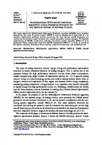
located such that no objective is favoured. • Attainment surface: the boundary in objective space formed by the obtained front, which separates the region dominated by the obtained solutions from the region that is not dominated [9]. Multiple attainment surfaces can be superimposed and interpreted probabilistically. For example, the 50% attainment surface identifies the region of objective space that is dominated by half of the given attainment surfaces, whereas the 100% attainment surface identifies the region dominated by every given attainment surface. Whereas generational distance and diversity complement one another, the hyper-volume metric represents a combined value that rewards both closeness to the Pareto optimal front, and the extent of the obtained non-dominated front. Importantly, the hyper-volume metric is more robust than either of the former two metrics [13, 2]. In order to calculate these metrics, we sample the Pareto optimal front 500 times, evenly spread with respect to the first objective. Smaller generational distance and diversity values, and larger hyper-volume values, indicate better performance. 4.4 Metrics Comparison Since attainment surfaces operate in objective space, they are more robust than numerical metrics (which attempt to reduce complex multi-dimensional data down to single numerical values). Figure 3 shows some 50% attainment surfaces, where curves closer to the origin indicate better performance for the minimisation problems considered.

ESP Aspect Population size (µ) Child population size (λ) Total generations Child population creation Encoding Recombination Ranking scheme Mutation

Truncation

Strategy/Setting 100. 100. 250. Since µ = λ, the child population is created by cloning the parent population and then applying the genetic operators. Direct concatenation of real numbers. Uniform crossover variant. Unique pairs of individuals randomly swap their decision variables and average their step-sizes. Goldberg’s non-dominated ranking procedure [10]. Mutation probability p = 1/m, with self adaptivep mutation rates using √ √ initial step size = 0.1, τ 0 = 0.5/ 2m, τ = 0.5/ 2 m. Mutations producing infeasible values are re-tried in the same direction. SPEA2 truncation, using the hyper-volume based truncation measure.

Table 2: The settings used by the implementation of ESP in this study, except where noted otherwise. However, the other metrics are better suited to numerical analysis techniques. In this study the mean difference between two unary metric distributions is taken as the test statistic. The significance of this observed difference is tested using randomisation testing [14] — if the observed result has arisen by chance, then it will not appear unusual in a distribution of results obtained via the random relabelling of samples. For this study, the randomisation test proceeds in the manner used by Purshouse and Fleming. Randomisation test results are easy to visualise and interpret, as shown in Figure 4(a). The histogram shows the distribution constructed by the 5000 randomised differences, and the solid black circle shows the observed difference. The five rows of results correspond to the five test problems, and the three columns correspond to the three metrics, generational distance, diversity, and hyper-volume respectively. To demonstrate that ESP is better than the algorithm to which it is compared, the observed result should appear to the left of the distribution for the first two metrics, and to the right of the distribution for hyper-volume.

5 The ESP Algorithm ESP is a generalised form of the traditional (µ + λ)-ES, its principal distinguishing feature being the use of a mutation probability setting. ESP also employs a new hypervolume based, parameterless and scaling-independent truncation measure to resolve ties during truncation. Table 2 gives the settings used by ESP in this study. 5.1 Mutation As already indicated, a key factor that distinguishes ESP from other ESs, and allows it to perform so well, is the fact that individuals are mutated based on a probability p. The mutation operator acts as follows: • Self adapt the strategy parameters. • Using the strategy parameters, mutate each decision variable with probability p per variable. When p = 1, this corresponds to the mutation scheme normally used in ESs. Although we have yet to optimise it, we have obtained excellent results with p = 1/m.

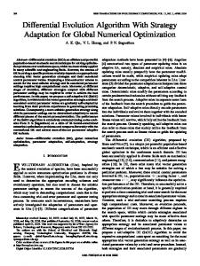
Although more complicated schemes exist, the self adaption scheme employed in this study is one described by B¨ack, Hammel, and Schwefel [3]. 5.2 Truncation The truncation procedure used is based on the truncation mechanism used by SPEA2. The main difference is that instead of employing a Euclidean distance-based nearest neighbour measure, we employ a new parameterless and scaling independent hyper-volume based intra-ranking mechanism. (Although there is an obvious connection, the hyper-volume based intra-ranking mechanism should not be confused with the hyper-volume performance metric.) Given a non-dominated front of individuals, the hypervolume value for an individual i, ωi , is equal to the product of the one-dimensional lengths to the next worse objective function value in the front for each objective, with the exception being for individuals with non-unique fitness vectors, each of which are assigned the worst possible hypervolume of zero. That is, in general the value for i is the hyper-volume of the region dominated with respect to the hypercube formed by the next worse individuals in each dimension. This is illustrated in Figure 2 for a two-objective minimisation problem. The extreme solutions ω0 and ω3 are assigned the value infinity. When selection is required between equally-ranked individuals from a population, the hyper-volume for each individual is calculated, and the individual with the smallest hyper-volume is discarded. This process is repeated until the desired population size is achieved, with hyper-volume values re-calculated in each iteration. Ties in hyper-volume values are resolved randomly. No normalisation or scaling is required for this measure, and we have found it both elegant to implement, and comparable in performance to nearest neighbour Euclidean distance based truncation.

6 Experiments and Results ESP was compared to a variety of other algorithms, including a version of ESP that has a mutation probability of 100% (ESP-1, simulating a more traditional ES), Purshouse

Figure 2: Calculation of the hyper-volume value for four individuals on a two-dimensional minimisation problem. and Fleming’s elitist, rank-based fitness sharing PF-MOGA, and SPDE (with no mutation). ESP was also compared to SPEA2 and NSGA-II, although results are limited since test data was only available for ZDT6 with increased dimensionality (m = 100), and using 100000 function evaluations. To make the comparison against SPEA2 and NSGA-II fair, we likewise increased the dimensionality of ZDT6 (denoted ZDT6-100), and allowed ESP to run for 1000 generations. Note that the test data available for each of the other algorithms on each problem does not always represent 35 distinct runs. This does not significantly influence the analysis. Figure 3 shows the 50% attainment surface achieved by each algorithm. We make the following observations: • The median performance of ESP is optimal or near optimal for all problems. • The median performance of ESP-1, in which decision variables are always mutated, is consistently poorer than that of ESP. • The median performance of ESP is clearly better than that of PF-MOGA on ZDT4, and somewhat better on ZDT1, ZDT2, and ZDT6. • The median performance of ESP is clearly better than that of SPDE on all problems. • The median performance of ESP is better than that of both NSGA-II and SPEA2 on ZDT6-100. Although the attainment surfaces show that ESP performs very well, it is important to consider the randomisation tests, wherein the statistical significance of the ESP’s performance can be empirically determined. The results of the randomisation tests are presented in Figure 4. We make the following observations: • For all problems and all metrics (barring diversity on ZDT3), the significance of incorporating probabilistic mutation into ESP (by comparison to ESP-1) is clear. • ESP outperforms PF-MOGA on all problems, except for diversity on ZDT3 (in addition to a small number of inconclusive comparisons). • ESP outperforms SPDE on all problems and all metrics. • ESP outperforms NSGA-II and SPEA2 on ZDT6-100

on all metrics. Some further comparison can be made against NSGA-II, in so far as Deb et al. [7] have presented the raw, averaged distance metric values for ZDT1–ZDT4, and ZDT6. Despite being a limited comparison, our tests indicate that the average generational distance values obtained by ESP are consistently equal to or (more often) better than those reported by Deb et al. (Note that the exact means by which Deb et al. calculate their distance metric, and in particular how the Pareto optimal front is sampled, is unclear, although any difference between metric implementations should be marginal.) By inference, we would expect a similar comparison to be upheld against SPEA2, given SPEA2 is reputedly comparable to NSGA-II. Nevertheless, without a direct comparison of the data, we cannot be conclusive on this. It is interesting to note that ESP has the most difficulty with ZDT4, although it still outperforms the other algorithms. To determine if further function evaluations would overcome any difficulty experienced by ESP on ZDT4, we ran it for 500 generations, with impressive results. On all 35 runs, ESP converged to the Pareto optimal front.

7 Conclusions Multi-objective optimisation is an important and difficult subject. To date the most success in this area has been seen with novel variations of GAs. However, we have demonstrated that the performance of an ES approach with probabilistic mutation exceeds that of state-of-the-art algorithms on a range of test problems under a variety of metrics. ESP’s most distinctive departure from conventional practice is the incorporation of mutation probability. Although it might be argued that self-adaptive mutation rates should override the need for mutation probabilities, the strength of our results suggests that this is not always the case. We plan to enhance ESP by incorporating mechanisms such as self adaptive mutation probabilities (not to be confused with mutation rates). We also plan to explore its performance on single-objective problems and on more difficult test problems, both constructed and real world ones. The test data employed in this paper is available for download from http://wfg.csse.uwa.edu.au/.

ZDT1

1.4

1.2

1

1

0.8

0.8

f2

1.2

f2

ZDT2

1.4

0.6

0.6

0.4

0.4

0.2

0.2

0

0 0.2

0

0.4

0.6

0.8

1

0.2

0

0.4

f1

0.6

0.8

1

f1

ZDT3

1.5

ZDT4

4.5 4

1

3.5 3

0.5

f2

f2

2.5 2 0 1.5 1

−0.5

0.5 −1

0 0

0.1

0.2

0.3

0.4

0.5

0.6

0.7

0.8

0.9

0.2

0

0.4

f1

0.6

0.8

1

f1

ZDT6

ZDT6−100

3.5 2 3

2.5

1.5

f2

f2

2 1 1.5

1 0.5 0.5

0

0 0.2

0.3

0.4

0.5

0.6

0.7

0.8

0.9

1

0.2

0.3

f1

0.4

0.5

0.6

0.7

0.8

0.9

1

f1

50% attainment surface for ESP 50% attainment surface for ESP−1 (not ZDT6−100) 50% attainment surface for PF−MOGA (not ZDT6−100) 50% attainment surface for SPDE (not ZDT6−100) 50% attainment surface for SPEA2 (ZDT6−100 only) 50% attainment surface for NSGA−II (ZDT6−100 only)

Figure 3: 50% attainment surfaces for ESP, ESP-1 (mutation probability 100%), PF-MOGA, SPDE, and SPEA2 and NSGA-II (100000 function evaluations, ZDT6 only, with m = 100). The latter two, SPEA2 and NSGA-II, are presented separately with ESP in the lower right plot on the graph labelled ZDT6-100. Extrema which lie outside the ranges of the axes have been omitted from the graphs.

Diversity

Hyper−volume

150

150

125

125

125

100

100

100

100

100

100

75

75

75

75

75

75

50

50

50

50

50

25

25

25

25

25

ZDT1

0 −0.15

−0.1

−0.05

0

0.05

0.1

0.15

frequency

150

125

−0.2

frequency

Diversity

150

125

0

ZDT2

Generational Distance

Hyper−volume

150

125

0

0 −0.5

−0.4

−0.3

−0.2

−0.1

0

0.1

0.2

−0.06

−0.04

−0.02

0

0.02

0.04

0.06

50

25

0 −0.0012

0.08

−0.0007

−0.0002

0.0003

0

0.0008

−0.5

−0.4

−0.3

−0.2

−0.1

0

0.1

0.2

−0.0015

150

150

150

150

150

150

125

125

125

125

125

125

100

100

100

100

100

100

75

75

75

75

75

75

50

50

50

50

50

25

25

25

25

25

ZDT2

0

0 −0.4

−0.3

−0.2

−0.1

0

0.1

0.2

frequency

ZDT1

frequency

Generational Distance 150

0

0 −0.6

−0.5

−0.4

−0.3

−0.2

−0.1

0

0.1

−0.1

−0.05

0

0.05

0.1

−0.0006

−0.0004

−0.0002

0

0.0002

0.0004

0.0005

0.0015

0.0025

0.0035

50

25

0 −0.0008

0.15

−0.0005

0

0.0006

−0.6

−0.5

−0.4

−0.3

−0.2

−0.1

0

0.1

0.2

0.3

−0.002

−0.001

0

0.001

0.002

0.003

0.004

175 150

150

150

150

125

125

100

100

125 150 125

125

100

100

100

ZDT3

100 75

frequency

frequency

125

ZDT3

75 75

75

50

50

50

75 75

50 50 50 25

25

25

25

25

0

0

0

0

0

frequency

−0.06

−0.04

−0.02

0

0.02

0.04

0.06

−0.08

−0.03

0.02

0.07

0.12

−0.04

−0.02

0

0.02

0.04

0.06

0.08

−0.0006

0.1

100

75

50

50

25

25

25

25

0

0

0

0

0 4

−0.4

−0.3

−0.2

−0.1

0

0.1

0.2

0.3

0.4

−0.03

−0.02

−0.01

0

0.01

0.02

0.03

0.04

0.05

−0.1

0.06

100

75

50

25

25

25

25

0

0

0

diff. between pop. means

0.3

−0.15

−0.1

−0.05

0

diff. between pop. means

0.05

0.1

0.15

0.2

0.25

−0.01

frequency

Generational Distance

Diversity 150

125

125

100

100

100

75

75

75

50

50

50

25

25

0

0 −0.005

0

0.005

0.01

0.0008

0.001

−0.001

−0.0005

0

0.0005

0.001

0.0015

0.002

25

0

0.015

−0.3

−0.2

−0.1

0

0.1

0.2

−0.008

−0.006

−0.004

diff. between pop. means

−0.002

0

0.002

0.004

0.006

0.008

0.01

diff. between pop. means

0.01

0.015

(b) ESP versus elitist, parameterless rank-based fitness sharing PF-MOGA.

Hyper−volume

150

125

−0.01

0.005

0.0006

observed difference

150

−0.015

0

diff. between pop. means

diff. between pop. means

(a) ESP versus ESP-1 (traditional mutation probability of 100%).

−0.02

−0.005

0.0004

50

0 −0.015

0.3

observed difference

−0.025

−0.0015

50

25

0.2

0.3

50

50

0.1

0.2

125

50

0

0.1

75

ZDT6

−0.1

0

100

75

−0.2

−0.1

125

100

75

−0.3

−0.2

75

125

100

75

0.0002

0 −0.3

100

125

100

0

25

0.1

125

125

−0.4

0.05

150

150

−0.5

0

150

150

1.5

−0.05

150

150

0

ZDT1

−0.0008 −0.0006 −0.0004 −0.0002

50

25

0.5

0.15

50

50

−0.5

0.1

125

50

−1.5

0.05

75

ZDT4

−2.5

0

100

75

−3.5

−0.05

125

100

75

2

0 −0.1

75

125

100

75

0

25

0.0004

100

125

100

−2

0.0002

125

125

−4

0

150

150

−6

−0.0002

150

150

−8

−0.0004

150

150

−10

ZDT6

−0.08

frequency

−0.1

frequency

ZDT4

frequency

−0.12

25

0 −0.8

−0.6

−0.4

−0.2

0

0.2

0.4

0.6

150

−0.01

−0.005

0

0.005

0.01

0.015

0.02

0.025

150 125

125

125

frequency

100

ZDT2

100

100 75

75

75 50

50

50

25

0

frequency

−0.04

ZDT3

−0.03

−0.02

−0.01

0

0.01

0.02

−0.6

−0.4

−0.2

0

0.2

150

150

125

125

125

100

100

100

75

75

75

50

50

25

25

−0.015

−0.01

−0.005

0

0.005

0.01

0.015

0.02

−0.1

−0.05

0

0.05

0.1

0.15

−0.01

−0.005

0

0.005

0.01

0.015

0.02

25

0 −0.08

−0.06

−0.04

−0.02

0

0.02

0.04

0.06

0.08

150

150

150

125

125

125

100

100

100

75

75

75

50

−0.15

50

0 −0.02

frequency

0 −0.8

150

0

ZDT4

25

0

50

Generational Distance

50

NSGA−II 25

25

0

25

0 −2.5

−2

−1.5

−1

−0.5

0

0.5

1

1.5

2

frequency

25

150

125

125

100

100

100

75

75

75

50

50

25

25

0

0

−0.4

−0.2

0

0.2

0.4

0.6

−0.015

−0.01

−0.005

0

0.005

0.01

0.015

0.02

0.025

150

125

125

125

100

100

100

75

75

75

50

50

50

25

25

25

0

0

0

−0.15

−0.1

−0.05

0

0.05

diff. between pop. means

0.1

0.15

−0.8

−0.6

−0.4

−0.2

0

diff. between pop. means

0.2

0.4

SPEA2

−0.06

−0.04

−0.02

0

0.02

0.04

diff. between pop. means

observed difference

(c) ESP versus SPDE (with no mutation).

0.06

0.08

frequency

frequency

150

−0.2

50

0 −0.6

150

−0.25

Hyper−volume

150

125

−1

ZDT6

Diversity

150

−0.8

−0.6

−0.4

−0.2

0

0.2

0.4

0.6

0.8

25

0 −0.25

−0.2

−0.15

−0.1

−0.05

0

0.05

0.1

0.15

−0.1

150

150

150

125

125

125

100

100

100

75

75

75

50

50

25

25

0

0 −1.2

−1

−0.8

−0.6

−0.4

−0.2

0

0.2

diff. between pop. means

0.4

0.6

−0.05

0

0.05

0.1

0.15

0.2

50

25

0 −0.25

−0.2

−0.15

−0.1

−0.05

0

diff. between pop. means

0.05

0.1

0.15

−0.1

−0.05

0

0.05

0.1

0.15

0.2

0.25

0.3

diff. between pop. means

observed difference

(d) ESP versus NSGA-II (top) and SPEA2 (bottom), using 100000 fitness evaluations on ZDT6-100 (m = 100).

Figure 4: Randomisation tests comparing ESP to (a) ESP-1, (b) PF-MOGA, (c) SPDE, and (d) NSGA-II and SPEA2. The columns, from left to right, show the histograms and observed results for generational distance, diversity, and hypervolume. ESP performs well when the observed result is to the left for the first two metrics, and to the right for the final metric. The unusual shapes of some histograms are caused by outlying results.

Acknowledgments We thank the Australian Research Council for their support. We thank Hussein Abbass for generating and providing test results for SPDE. We thank Robin Purshouse (www.shef.ac.uk/acse/research/students/r.c.purshouse) and Eckart Zitzler (www.tik.ee.ethz.ch/˜zitzler/testdata.html) for making the results for their algorithms available online.

Bibliography [1] H. A. Abbass. The Self-adaptive Pareto Differential Evolution algorithm. In D. B. Fogel et al., editor, CEC’02, volume 1, pages 831–836. IEEE, 2002.

[11] J. Knowles and D. Corne. Approximating the nondominated front using the Pareto archived evolution strategy. Evolutionary Computation, 8(2):149–172, 2000. [12] J. Knowles and D. Corne. M-PAES: A memetic algorithm for multiobjective optimization. In CEC’00, volume 1, pages 325–332. IEEE, 2000. [13] J. Knowles and D. Corne. On metrics for comparing nondominated sets. In D. B. Fogel et al., editor, CEC’02, volume 1, pages 711–716. IEEE, 2002. [14] B. F. J. Manly. Randomization, Bootstrap and Monte Carlo Methods in Biology. Chapman & Hall, 1991.

[2] K. H. Ang, G. Chong, and Y. Li. Preliminary statement on the current progress of multi-objective evolutionary algorithm performance measurement. In D. B. Fogel et al., editor, CEC’02, volume 2, pages 1139–1144. IEEE, 2002.

[15] R. C. Purshouse and P. J. Fleming. The MultiObjective Genetic Algorithm applied to benchmark problems — an analysis. Research Report 796, University of Sheffield, Dept of Automatic Control and Systems Engineering, UK, 2001.

[3] T. B¨ack, U. Hammel, and H-P. Schwefel. Evolutionary computation: Comments on the history and current state. IEEE Trans. on Evolutionary Computation, 1(1):3–16, 1997.

[16] R. C. Purshouse and P. J. Fleming. Elitism, sharing, and ranking choices in evolutionary multi-criterion optimisation. Research Report 815, University of Sheffield, Dept of Automatic Control and Systems Engineering, UK, 2002.

[4] L. Barone, L. While, and P. Hingston. Designing crushers with a multi-objective evolutionary algorithm. In W. B. Langdon et al., editor, GECCO-2002, pages 995–1002. Morgan Kaufmann Publishers, 2002. [5] D. B¨uche, P. Stoll, R. Dornberger, and P. Koumoutsakos. Multiobjective evolutionary algorithm for the optimization of noisy combustion processes. IEEE Trans. on Systems, Man, and Cybernetics — Part C: Applications and Reviews, 32(4):460–473, 2002. [6] L. Costa and P. Oliveira. An evolution strategy for multiobjective optimization. In D. B. Fogel et al., editor, CEC’02, volume 1, pages 97–102. IEEE, 2002. [7] K. Deb, A. Pratap, S. Agarwal, and T. Meyarivan. A fast and elitist multiobjective genetic algorithm: NSGA-II. IEEE Trans. on Evolutionary Computation, 6(2):182–197, 2002. [8] C. M. Fonseca and P. J. Fleming. Genetic algorithms for multiobjective optimization: Formulation, discussion and generalization. In S. Forrest, editor, Proceedings of the Fifth International Conference on Genetic Algorithms, pages 416–423. Morgan Kaufmann Publishers, 1993. [9] C. M. Fonseca and P. J. Fleming. On the performance assessment and comparison of stochastic multiobjective optimizers. In H-M. Voigt et al., editor, PPSN IV, volume 1141 of LNCS, pages 584–593. SpringerVerlag, 1996. [10] D. E. Goldberg. Genetic Algorithms in Search, Optimization & Machine Learning. Addison-Wesley, 1989.

[17] R. C. Purshouse and P. J. Fleming. Why use elitism and sharing in a multi-objective genetic algorithm? In W. B. Langdon et al., editor, GECCO-2002, pages 520–527. Morgan Kaufmann Publishers, 2002. [18] R. C. Purshouse and P. J. Fleming. An adaptive divide-and-conquer methodology for evolutionary multi-criterion optimisation. In C. M. Fonseca et al., editor, EMO 2003, volume 2632 of LNCS, pages 133– 147. Springer-Verlag, 2003. [19] D. A. Van Veldhuizen. Multiobjective Evolutionary Algorithms: Classifications, Analyses, and New Innovations. PhD thesis, Air Force Inst of Technology, Wright-Patterson AFB, Ohio, 1999. [20] E. Zitzler. Evolutionary Algorithms for Multiobjective Optimization: Methods and Applications. PhD thesis, Swiss Federal Inst of Technology (ETH) Zurich, 1999. [21] E. Zitzler, K. Deb, and L. Thiele. Comparison of multiobjective evolutionary algorithms: Empirical results. Evolutionary Computation, 8(2):173–195, 2000. [22] E. Zitzler, M. Laumanns, and L. Thiele. SPEA2: Improving the strength Pareto evolutionary algorithm for multiobjective optimization. In K. C. Giannakoglou et al., editor, EUROGEN 2001, pages 95–100. International Center for Numerical Methods in Engineering (CIMNE), Barcelona, Spain, 2001. [23] E. Zitzler and L. Thiele. Multiobjective evolutionary algorithms: A comparative case study and the strength Pareto approach. IEEE Trans. on Evolutionary Computation, 3(4):257–271, 1999.