2007 International Nuclear Atlantic Conference - INAC 2007 Santos, SP, Brazil, September 30 to October 5, 2007 ASSOCIAÇÃO BRASILEIRA DE ENERGIA NUCLEAR - ABEN ISBN: 978-85-99141-02-1
AN EXPERIMENTAL AND NUMERICAL SIMULATION FOR THE PREDICTION OF STRATIFIED FLOWS IN NUCLEAR REACTORS Hugo Cesar Rezende1, Moysés Alberto Navarro1, André A. Campagnole dos Santos2, Hermes Carvalho2 1
Centro de Desenvolvimento da Tecnologia Nuclear (CDTN / CNEN - MG) Rua. Professor Mário Werneck, s/n – Cidade Universitária 30123-970 Belo Horizonte, MG
[email protected] [email protected] 2
Departamento de Engenharia Mecânica – DEMEC Universidade Federal de Minas Gerais - UFMG Av. Antônio Carlos, 6627 31271-901 Belo Horizonte, MG
[email protected] .br
[email protected]
ABSTRACT Thermal stratification and striping have been observed in piping systems of nuclear power plants. The phenomena play an important role in the piping integrity, due to the appreciable thermal stresses that may induce undesirable failures and deformations of the piping. To obtain some understanding on these phenomena, experimental and numerical programs have been set up at CDTN/CNEN. This paper reports a thermal-hydraulic assessment of stratified flow, under conditions similar to the steam generator injection nozzle of a pressurized water reactor. Numerical results obtained with a commercial finite volume CFD code, CFX-10.0, are presented and compared with experimental data. Experiments performed with two flow rates that correspond to the Froude numbers of 0.146 and 0.433 were simulated. The RANS two equations RNG k-ε turbulence model was used in the simulation. Both results confirmed the occurrence of thermal stratification under the simulated conditions, with reasonable agreement with one another.
1. INTRODUCTION One phase thermally stratified flow is the condition that occurs in a piping, where two different layers of the same liquid at great temperature difference flow separately, without appreciable mixing due to low flow velocities and density difference. This condition results in a varying temperature distribution in the pipe wall and in an excessive differential expansion of the upper and lower parts of the pipe threatening the integrity of the piping system. Some safety related piping systems connected to reactor coolant systems in operating nuclear power plants are known to be potentially susceptible to thermally stratified flows. Piping systems of PWR-plants typically related with thermal stratification are pressurizer surge lines, emergency core cooling lines, residual heat removal lines and also some segments of the main piping of the primary and secondary cooling loops, like the hot and cold legs in the primary and the steam generator feedwater piping in the secondary, (Häfner, 1990, and Schuler and Herter, 2004). Temperature differences of about 200 °C can be found in a narrow
band around the hot and cold water interface. To assess potential piping damage due to thermal stratification, it is necessary to determine the transient temperature distributions in the pipe wall. The driving parameter considered to characterize flow under stratified regime due to difference in specific masses is the Froude number, given by: Fr =
U0
(gD Δρ /ρ 0 )1 2
(1)
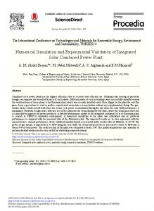
where U0 is the average velocity of the injected water in [m/s], g is the acceleration of the gravity in [m/s2], D is the inner diameter of the tube in [m], Δρ is the difference between the densities of the hot and cold water in [kg/m3] and ρ0 is the density of the cold water in [kg/m3]. This paper summarizes an experimental and a numerical methodology developed for the simulation of one phase thermally stratified flow in a nuclear reactor steam generator nozzle. 2. EXPERIMENTAL METHODOLOGY Figure 1 shows a diagram of the experimental facility test section. A vessel simulates the steam generator tank and a horizontal-to-vertical stainless steel piping (D = 0.1223 m) simulates the steam generator injection nozzle. In a typical experiment, both the vessel and the piping are filled with hot water and cold water is injected with a low flow rate through a bottom nozzle at the end of the vertical pipe. The water leaves the piping through eleven upper holes at the horizontal segment of pipe inside the vessel.
Measuring stations
Figure 1. Diagram of the experimental facility test section and thermocouple distribution on its measuring stations 1, 2, 3 and A. INAC 2007, Santos, SP, Brazil.
Wall and fluid temperatures are measured with type K thermocouples 0.5 mm in diameter, distributed in three measuring stations (1, 2, 3). In each measuring station fluid thermocouples are positioned along the tube vertical diameter and along the inner wall, 3 mm away from the wall. Wall thermocouples were brazed along the outer wall. Two thermocouples installed at position “A” aim to synchronize the experimental and numerical cold water front arrival. The water temperature was also measured with type K thermocouples in the injection piping and in the cold water tank. The measurement of the injected water flow rate was performed by an orifice plate and the pressure of the system by a gauge pressure transducer. This paper presents results of two tests and comparisons with numerical simulations. Table 1 shows the setting parameters values for both tests.
Table 1. Setting parameters for the two tests. Fr
Flow rate [kg/s]
P [bar]
Thot [oC]
Tcold [oC]
0.146 0.433
0.756 1.878
21.2 10.0
219.2 185.6
31.7 27.6
0.5
2
2
0.03 δ1 1- Global uncertainty
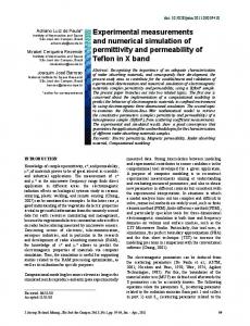
3. NUMERICAL METHODOLOGY Two main simplifications in the geometry of the test section, hachured in Fig. 1, were assumed in the simulations: a) the omission of the flanges and some geometric details at the entrance of the test section; b) the omission of the vessel, assuming that the same boundary condition was adopted in the rest of the test section (adiabatic) for the pipe contained in the vessel. The numerical simulation used a commercial CFD code CFX 10.0 (ANSYS CFX) based on the finite volume method. Two simulation domains were created: one solid, corresponding to the pipe, and one fluid for the water in its interior. A vertical symmetry plane along the pipe was adopted to reduce the geometry in one half, reducing the mesh size and minimizing processing time. An unstructured mesh with tetrahedral elements was defined inside the pipe. Two layers of prismatic structured volumes were built close to the surfaces in the solid and fluid domains. Located mesh refinement in the regions of the inlet nozzle and of the outlet holes were necessary due to the local contraction and expansion of fluid that generate high pressure and speed gradients in these regions. Simulations were performed with several refinement levels before adopting a pattern of appropriate mesh. Figure 2 presents details of the mesh adopted for the simulation, with 1,875,318 elements in the fluid domain and 606,848 elements in the solid domain. The initial conditions used for the numerical simulation were the same obtained in the experiment for the piping wall temperature, hot and cold water temperature and internal pressure. The two experimental flow rates presented in Tab. 1 were simulated. Water properties like density, viscosity and thermal expansivity were adjusted by regression as function of temperature with data extracted from the Table IAPWS-IF97, in the simulation range (25 oC to 221 oC). No heat transfer was considered through the external wall of the pipe (adiabatic wall boundary condition). The RANS - Reynolds Averaging Navier-Stokes equations, the two
INAC 2007, Santos, SP, Brazil.
equations of the RNG k-ε turbulence model, with scalable wall functions, the full buoyancy model and the total energy heat transfer model with the viscous work term were solved. The simulations were performed using parallel simulation on two personal computers Pentium IV HT with 3 Ghz processor, 4 Gb of RAM and 100 Mbps ethernet card. Time step, total transient time and total processing time of each flow rate simulated are presented in Tab. 2. Table 2. Simulation characteristics Flow rate [kg/s]
Time step [s]
Total transient [s]
Total processing time [h]
0.756 1.878
0.05 - 0.1 0.005 - 0.048
183 50
696 715 A
A
Wall Section “A-A”
Figure 2. Mesh details. 4. RESULTS Figure 3 shows the experimental and numerical temperature behaviors in the lowest thermocouple positions of the vertical probes in the measuring stations 1 (T1S08), 2 (T2S08) and 3 (T3S05), respectively, for both flow rates evaluated. The temperatures fall successively at probes 1, 2 and 3, due to the arrival of the cold water front at each probe position. The figure shows that, despite the synchronization between the experimental and numerical results (here adjusted to experiment) at position A, the arrival of the cold water front at the lower thermocouple positions obtained with the numerical simulation occurred earlier than detected experimentally. The difference between both results increases with the distance from position A. At measuring station 3, the difference reaches 3 s for the lowest flow rate (0.756 kg/s) and 2 s for the highest flow rate (1.878 kg/s). The figure shows also that the temperature drop due to the arrival of the cold water front is more abrupt in the numerical results than in the experimental results. INAC 2007, Santos, SP, Brazil.
Flow rate 0.756 kg/s: Vertical measuring probes 2 3 1 T2S08
T1S08 23.75 mm
150
Temperature [ºC]
Temperature [ºC]
200
T3S05
100 50 0 0
25
50
75 Time [s]
100
125
Flow rate 1.878 kg/s:
200 180 160 140 120 100 80 60 40 20 0
150
EXP CFX T1S08 T2S08 T3S05
0
10
20 Time [s]
30
40
50
Figure 3. Temperature evolutions along the lower region of the horizontal pipe for two flow rates. Flow rate 0.756 kg/s:
61.15 mm
150
180 Temperature [ºC]
Temperature [ºC]
200
100 50
Flow rate 1.878 kg/s:
200
Vertical measuring probes 2 3 1 T1S05 T2S04 T3S02
160 140 120 100 80 60
T1S05 T2S04 T3S02
40 20
0
0
0
25
50
75 Time [s]
100
125
150
0
EXP CFX
10
20 Time [s]
30
40
50
Figure 4. Temperature evolutions along the middle region of the horizontal pipe for two flow rates. Figure 4 shows the temperature evolutions at middle high thermocouple positions at the three measuring stations for the two flow rates. At the flow rate of 0.756 kg/s the experimental results show a successive initial cooling in thermocouples T1S05, T2S04 and T3S02 followed by a sudden successive cooling in thermocouples T3S02, T2S04 and T1S05. The first and initial cooling was not observed in the numerical simulation. The numerical results show that, for the flow rate of 0.756 kg/s, the cold water front hits the wall at the end of the horizontal pipe and a part of the cold water returns through the pipe in the opposite direction as a second cold water front. Figure 5 shows the cold water front evolution for the flow rate of 0.756 kg/s obtained with CFX. A change in the direction of the cold water front after it reaches the end of the tube can be observed. For the flow rate of 1.878 kg/s this return was not predicted by CFX. The thermocouples T1S05, T2S04 and T3S02 were cooled successively, as shown in Fig. 4. For the flow rate of 1.878 kg/s, the cold water reaches the orifices and goes out of the test section in a preferential way, trapping hot water at the top of the horizontal pipe. The “imprisoned” hot water maintains a circulating motion while the level of the cold water increases, as can be seen in Fig. 5.
INAC 2007, Santos, SP, Brazil.
Flow rate 0.756 kg/s
Flow rate 1.878 kg/s
t = 23s
t = 12.5s
t = 30s
t = 16.5s
t = 35s
t = 20.5s
t = 40s
t = 23.5s
t = 48s
t = 26.5s
t = 52s
t = 30.5s
t = 64s
t = 42.5s
[°C]
[°C]
Figure 5. Temperature contours at different times for both flow rates. 220
o T [ C]
165 110
Flow rate [kg/s]: CFX EXP 0.756 1.878
55 0 -0.061
-0.031
-0.001
0.029
0.059
R [m]
Figure 6. Temperature distributions along the vertical diameter of measuring station 1. Figure 6 shows the temperature distributions along the vertical diameter of the measuring station 1. Data were taken at 59 s for flow rate 0.756 kg/s and 30 s for flow rate 1.878 kg/s. The high temperature gradient defines a pronounced thermal stratification for the lower flow rate. For the higher flow rate the temperature gradient is smoother. Figure 7 shows the temperature evolution in three positions of thermocouples at the middle height of measuring station 2 for both flow rates. The positions correspond to thermocouple T2S04 at the center of the tube, thermocouple T2I15, 3 mm away from the inside wall, and thermocouple T2E11 brazed on the outside wall. Both numerical and experimental evolutions show small temperature differences between thermocouple positions T2S04 and T2I15 but differences superior to 50 oC between these temperatures and the external surface temperatures (T2E11).
INAC 2007, Santos, SP, Brazil.
Flow rate 0.756 kg/s:
180 160 Temperature [ºC]
200 Temperature [ºC]
Flow rate 1.878 kg/s:
200
150 100 EXP CFX T2I15 T2S04 T2E11
50
140 120 100 80 60
T2S04
40 20
61.15 mm
T2I15
T2E11
0
0 0
25
50
75 Time [s]
100
125
0
150
10
20 Time [s]
30
40
50
Figure 7. Temperature evolution at the middle high at measuring station 2 for both flow rates. Figure 8 shows the evolution of the temperature difference, DT, between the average temperature on the highest part of the horizontal tube and the average temperature on the lowest part of the tube. These averages were obtained from the positions of the highest wall thermocouples at measuring stations 1 and 2 and from the lowest positions of the wall thermocouples at the same measuring stations. The temperature differences, DT, for the highest and lowest inside thermocouples, 3 mm from the wall, are also shown in Fig. 8. Temperature differences up to ≈170 oC (0.756 kg/s) and ≈140 oC (1.878 kg/s) between the upper and lower internal averages and up to ≈120 oC (0.756 kg/s) and ≈100 oC (1.878 kg/s) between the upper and lower external averages were observed for both numerical and experimental simulations. Flow rate 1.878 kg/s:
Flow rate 0.756 kg/s:
180
160
160
140
140
120
100
o DT [ C]
o
DT [ C]
120 80 60
Internal: External:
40
20
40
60 Time [s]
60
20
0 0
80
40
EXP CFX
20
100
80
100
0 0
10
20
Time [s]
30
40
50
Figure 8. Temperature difference between the upper and the lower part of the horizontal pipe
5. CONCLUSIONS The one phase thermal stratification was simulated numerically and experimentally in a piping system similar to the steam generator injection nozzle at the secondary loop of a Pressurized Water Reactor (PWR). The simulations were carried out with Froude numbers
INAC 2007, Santos, SP, Brazil.
close to nuclear reactors operation (Fr ≅ 0.146 and 0.433) and a great temperature gradient was obtained, characterizing thermal stratification. Despite the simplifications assumed in the numerical simulations the results presented a satisfactory agreement with the experimental results in the lower region of the horizontal pipe. In the upper region, the temperature drops due to the cold water front arrival calculated by the CFX 10.0 occured earlier than those obtained experimentally. The experimental thermocouple distribution together with the data collecting frequency were enough to detect the oscillation of the interface between cold and hot water layers (striping). These oscillations were also obtained in the numerical simulation. In spite of the differences between the experimental and numerical results, the behaviors of the parameters observed experimentally could be explained through the numerical simulations. The employed numerical methodology can be considered a good additional tool for predicting thermal stratification behavior and planning experiments. Simulations using better mesh and time step refinement with a LES (Large Eddy Simulation) methodology could further enlighten the physical behavior of thermal stratification and striping in nuclear reactor piping.
REFERENCES 1. CFX-10.0, “User manual”, ANSYS-CFX (2005). 2. Häfner, W., “Thermische Schichit-Versuche im horizontalen Rohr”, Kernforschungszentrum Karlsruhe GmbH, Karlsruhe, Germany , 238 p (1990). 3. Schuler, X. and Herter, K. H., “Thermal fatigue due to stratification and thermal schock loading of piping”, 30th MPA – Seminar in conjunction with the 9th German-Japanese Seminar, Stuttgart, Oct. 6. and 7., pp. 6.1 – 6.14 (2004).
INAC 2007, Santos, SP, Brazil.